|
Most of the available commercial traffic simulation software provides advanced
user-friendly graphic user interfaces with flexible and powerful graphic
editors to assist analysts in the model-building process.
This reduces the number of errors.
There are a number of manual ways to quantify the error associated with every
parameter while calibrating them.
Some of the common measures of error and their expressions are discussed below.
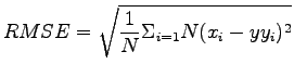
- Root mean square error
 |
(1) |
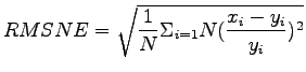
- Root mean squared normalized error
 |
(2) |
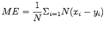
- Mean error
 |
(3) |
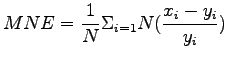
- Mean normalized error
 |
(4) |
where,  is the ith measured or simulated value, is the ith measured or simulated value,  is the ith observed
value is the ith observed
value
The above error measures are useful when applied separately to measurements at
each location instead of to all measurements jointly.
They indicate the existence of systematic bias in terms of under or over
prediction by the simulation model.
Taking into account that the series of measurements and simulated values can be
collected at regular time intervals, it becomes obvious that they can be
interpreted as time series and, therefore, used to determine how close the
simulated and the observed values are.
Thus it can be determined that how similar both time series are.
On the other hand, the use of aggregated values to validate a simulation seems
contradictory if one takes into account that it is dynamic in nature, and thus
time dependent.
Theil defined a set of indices aimed at this goal and these indices have been
widely used for that purpose.
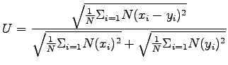
The first index is Theil's indicator, U (also called Theil's inequality
coefficient), which provides a normalized measure of the relative error that
reduces the impact of large errors:
 |
(5) |
The global index U is bounded,
 , with U = 0 for a perfect fit
and = for i = 1 to N, between observed and simulated values.
For , with U = 0 for a perfect fit
and = for i = 1 to N, between observed and simulated values.
For
 , the simulated series can be accepted as replicating the
observed series acceptably well.
The closer the values are to 0, the better will be the model.
For values greater than 0.2, the simulated series is rejected.
The observed and simulated values obtained using Model 1 and Model 2 are given
in Table below. , the simulated series can be accepted as replicating the
observed series acceptably well.
The closer the values are to 0, the better will be the model.
For values greater than 0.2, the simulated series is rejected.
The observed and simulated values obtained using Model 1 and Model 2 are given
in Table below.
Table 1:
Observed and Simulated values
| |
Simulated values, x |
| Observed values, y |
Model 1 |
Model 2 |
| 0.23 |
0.2 |
0.27 |
| 0.46 |
0.39 |
0.5 |
| 0.67 |
0.71 |
0.65 |
| 0.82 |
0.83 |
0.84 |
- Comment on the performance of both the models based on the following
error measures - RMSE, RMSNE, ME and MNE.
- Using Theil's indicator, comment on the acceptability of the models.
- Using the formulas given below (Equations 16.4, 16.5, 16.6, 16.7), all
the four errors can be calculated. Here N = 4.
Tabulations required are given below.
Table 2:
Error calculations for Model 1
| Model 1 |
( ) ) |
(
 ) ) |
 |
 |
| -0.030 |
-0.130 |
0.0009 |
0.0170 |
| -0.070 |
-0.152 |
0.0049 |
0.0232 |
| 0.040 |
0.060 |
0.0016 |
0.0036 |
| 0.010 |
0.012 |
0.0001 |
0.0001 |
 = -0.050 = -0.050 |
= -0.211 |
= 0.0075 |
= 0.0439 |
| ME = 0.013 |
MNE = 0.053 |
RMSE = 0.043 |
RMSNE = 0.105 |
Table 3:
Error calculations for Model 2
| Model 2 |
| () |
(
) |
|
|
| 0.040 |
0.174 |
0.0016 |
0.0302 |
| 0.040 |
0.087 |
0.0016 |
0.0076 |
| -0.020 |
-0.030 |
0.0004 |
0.0009 |
| 0.020 |
0.024 |
0.0004 |
0.0006 |
| = 0.080 |
= 0.255 |
= 0.0040 |
= 0.0393 |
| ME = 0.020 |
MNE = 0.064 |
RMSE = 0.032 |
RMSNE = 0.099 |
Comparing Model 1 and Model 2 in terms of RMSE and RMSNE, Model 2 is better. But with respect to ME and MNE, Model 1 is better.
- Theil's indicator
The additional tabulations required are as follows:
Table 4:
Theil's indicator calculation
 |
|
| Model 1 |
Model 2 |
 |
| 0.04 |
0.0729 |
0.0529 |
| 0.1521 |
0.25 |
0.2116 |
| 0.5041 |
0.4225 |
0.4489 |
| 0.6889 |
0.7056 |
0.6724 |
| = 1.3851 |
= 1.451 |
= 1.3858 |
The value of Theil's indicator is obtained as:
For Model 1, U = 0.037 which is  0.2, and
For Model 2, U = 0.027 which is 0.2.
Therefore both models are acceptable. 0.2, and
For Model 2, U = 0.027 which is 0.2.
Therefore both models are acceptable.
|
|