The basic steps involved in the development are same irrespective of the type
of model. The different activities involved are the following.
- Define the problem and the model objectives
- Define the system to be studied - Roadway, Vehicle and Driver
characteristics
- Model development
- Model calibration
- Model verification
- Model validation
- Documentation
The most significant steps among the above are described with the help of
stating the procedure for developing a microscopic model.
The framework of a model consists of mainly three processes as mentioned below.
- Vehicle generation
- Vehicle position updation
- Analysis
The flow diagram of a microscopic traffic simulation model is given in Figure
16.2. The basic structure of a model includes various component models like car
following models like car following models, lane changing models etc. which
come under the vehicle position updation part.
In this chapter, the vehicle generation stage is explained in detail.
The vehicles can be generated either according to the distributions of
vehicular headways or vehicular arrivals.
Headways generally follow one of the following distributions.
- Negative Exponential Distribution (Low flow rate)
- Normal Distribution (High flow rate)
- Erlang Distribution (Intermediate flow rate)
The generation of vehicles using negative exponential distribution is
demonstrated here.
The probability distribution function is given as follows.
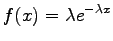 |
(1) |
From the above equation, the expression for exponential variate headway X can
be derived as:
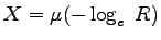 |
(2) |
where,  is the mean headway, R is the random number between 0 and 1 is the mean headway, R is the random number between 0 and 1
Figure 1:
Flow diagram of a Microscopic traffic simulation model
|
|
Random number generation is an essential part in any stochastic simulation
model, especially in vehicle generation module.
Numerous methods in terms of computer programs have been devised to generate
random numbers which appear to be random.
This is the reason why some call them pseudo-random numbers.
Therefore headways can be generated using the above expression by giving a
random number and the mean headway as the input variables.
In a similar way, the vehicular arrival pattern can be modeled using Poisson's
distribution.
The probability mass function is given as:
 |
(3) |
where, p(x) is the probability of x vehicle arrivals in an interval t,
 is the mean arrival rate of vehicles
If the probability of no vehicle in the interval t is given as p(0), then this
probability is same as the probability that the headway greater than or equal
to t.
Given flow rate is 900 veh/hr. Simulate the vehicle arrivals for 1 min using
negative exponential distribution.
Step 1: Calculate the mean headway is the mean arrival rate of vehicles
If the probability of no vehicle in the interval t is given as p(0), then this
probability is same as the probability that the headway greater than or equal
to t.
Given flow rate is 900 veh/hr. Simulate the vehicle arrivals for 1 min using
negative exponential distribution.
Step 1: Calculate the mean headway
 .
Step 2: Generate the random numbers between 0 and 1.
Step 3: Calculate the headways
and then estimate the cumulative headways. The calculations are given in
Table 1 .
Step 2: Generate the random numbers between 0 and 1.
Step 3: Calculate the headways
and then estimate the cumulative headways. The calculations are given in
Table 1
Table 1:
Vehicle arrivals using Negative exponential distribution
| Veh. No. |
R |
X |
Arrival time (sec) |
| 1 |
0.73 |
1.23 |
1.23 |
| 2 |
0.97 |
0.14 |
1.37 |
| 3 |
0.27 |
5.26 |
6.63 |
| 4 |
0.44 |
3.25 |
9.88 |
| 5 |
0.52 |
2.63 |
12.51 |
| 6 |
0.77 |
1.05 |
13.55 |
| 7 |
0.43 |
3.39 |
16.94 |
| 8 |
0.81 |
0.84 |
17.79 |
| 9 |
0.08 |
9.96 |
27.75 |
| 10 |
0.74 |
1.18 |
28.93 |
| 11 |
0.53 |
2.58 |
31.51 |
| 12 |
0.81 |
0.83 |
32.34 |
| 13 |
0.15 |
7.46 |
39.80 |
| 14 |
0.44 |
3.26 |
43.06 |
| 15 |
0.29 |
5.02 |
48.08 |
| 16 |
0.68 |
1.56 |
49.63 |
| 17 |
0.05 |
12.09 |
61.72 |
|
The hourly flow rate in a road section is 900 veh/hr. Use Poisson distribution
to model this vehicle arrival for 10 min.
Step 1: Calculate the no. of vehicles arriving per min.
= 900/60 = 15 veh/min.
Step 2: Calculate the probability of 0, 1, 2, ... vehicles per minute using
Poisson distribution formula.
Also calculate the cumulative
probability as shown below.
Step 3: Generate random numbers from 0 to 1. Using the calculated cumulative
probability values, estimate the no. of vehicles arriving in that interval as
shown in Table below.
Table 2:
Calculation of probabilities using Poisson distribution
| n |
p(x=n) |
p(x<=n) |
| 0 |
0.000 |
0 |
| 1 |
0.000 |
0.000 |
| 2 |
0.000 |
0.000 |
| 3 |
0.000 |
0.000 |
| 4 |
0.001 |
0.001 |
| 5 |
0.002 |
0.003 |
| 6 |
0.005 |
0.008 |
| 7 |
0.010 |
0.018 |
| 8 |
0.019 |
0.037 |
| 9 |
0.032 |
0.070 |
| 10 |
0.049 |
0.118 |
| 11 |
0.066 |
0.185 |
| 12 |
0.083 |
0.268 |
| 13 |
0.096 |
0.363 |
| 14 |
0.102 |
0.466 |
| 15 |
0.102 |
0.568 |
| 16 |
0.096 |
0.664 |
| 17 |
0.085 |
0.749 |
| 18 |
0.071 |
0.819 |
| 19 |
0.056 |
0.875 |
| 20 |
0.042 |
0.917 |
|
Table 3:
Vehicle arrivals using Poisson distribution
| t (min) |
R |
n |
| 1 |
0.231 |
11 |
| 2 |
0.162 |
10 |
| 3 |
0.909 |
19 |
| 4 |
0.871 |
18 |
| 5 |
0.307 |
12 |
| 6 |
0.008 |
6 |
| 7 |
0.654 |
15 |
| 8 |
0.775 |
17 |
| 9 |
0.632 |
15 |
| 10 |
0.901 |
20 |
| |
|
143 |
|
Here the total number of vehicles arrived in 10 min is 143 which is almost same
as the vehicle arrival rate obtained using negative exponential distribution.
|
![\includegraphics[width = 14cm]{qfflowdiagram}](img4.png)