We define
 |
(5.34) |
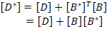
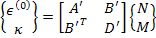
We make a note that  and we can write and we can write
Using the above definitions, Equation (5.32) and Equation (5.33) can be written together as
 |
(5.35) |
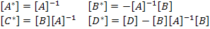
The above equation is called as partially inverted constitutive equation for laminate. From the second of the above equation we write
 |
(5.36) |
Putting this in Equation (5.35) we can get for  as as
 |
(5.37) |
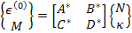
Let us define
 |
(5.38) |
Combining Equations (5.37) and (5.36) and using the definitions in Equation (5.38), we can write
 |
(5.39) |
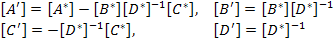
This equation is the fully inverted form of laminate constitutive equation. Using Equation (5.34) in Equation (5.38) we can write the above equation in terms of A, B and D matrices as
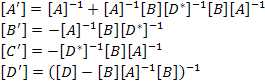 |
(5.40) |
From this equation it is easy to deduce that
 |
(5.41) |
The full matrix  is symmetric. This also follows from the fact that this is an inverse of a symmetric matrix, that is is symmetric. This also follows from the fact that this is an inverse of a symmetric matrix, that is  , and the inverse of a symmetric matrix is also a symmetric matrix. , and the inverse of a symmetric matrix is also a symmetric matrix.
Equation (5.28) and Equation (5.39) are very important equations in laminate analysis. These equations relate the mid-plane strains and curvatures with resultant in-plane forces and moments and vice versa. |