Next: 4.1 Algorithm (Predictor-corrector Method)
Up: lec1
Previous: Example
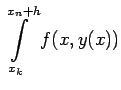
In section 1,2 during the course of the discussion on the Euler's
Algorithm, the approximated value of
is
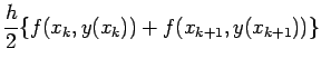
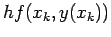 . On the other hand we could have also
considered its approximate value by
we could have thought of it to solve the IVP (numerically) by
defining the approximations
. On the other hand we could have also
considered its approximate value by
we could have thought of it to solve the IVP (numerically) by
defining the approximations
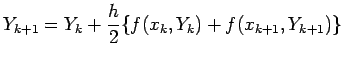 |
4.1 |
with  and
and
 . An
equation of the type (4.1) for
. An
equation of the type (4.1) for  is called an implicit
equation for
is called an implicit
equation for  . On many occasions solving of (4.1) could
be too tough and so we so resort to (numerical) approximate value
for
. On many occasions solving of (4.1) could
be too tough and so we so resort to (numerical) approximate value
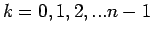
for  . Note here we are concentrating more on computing
, for a fixed
. Note here we are concentrating more on computing
, for a fixed  between 0 and n-1. To start with we let
 and let
  and define , for k=0,1,2...
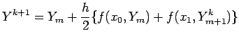 |
4.2 |
Essentially we are trying to iterate for
 . We need to step this iteration at some stage and the "find
value " of
. We need to step this iteration at some stage and the "find
value " of  is designated as . One method of
stopping the iteration is when
is "small" (small have means that the absolute value of the ratio
is lesser then an assigned (previously) small number.) We repeat
the process with in place of
is designated as . One method of
stopping the iteration is when
is "small" (small have means that the absolute value of the ratio
is lesser then an assigned (previously) small number.) We repeat
the process with in place of  and
and  in place of
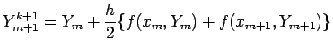
 . In general (4.1) allows us to define
and define
for k=0,1,2...and m=0,1,2,...n.
. In general (4.1) allows us to define
and define
for k=0,1,2...and m=0,1,2,...n.
The iterated values
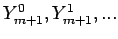 are called the inner
iterations for
are called the inner
iterations for  . Some more terminologies: Normally an
explicit method like Euler's method or R-K methods are known as
open type method or algorithm. They are readily available for
computation and the starters are known. On the other hand implicit
method as described by (4.2) is called closed type. Many a times
it may happen that the starters for the(approximate solution) for
closed type method is obtained from the open type one. The starter
. Some more terminologies: Normally an
explicit method like Euler's method or R-K methods are known as
open type method or algorithm. They are readily available for
computation and the starters are known. On the other hand implicit
method as described by (4.2) is called closed type. Many a times
it may happen that the starters for the(approximate solution) for
closed type method is obtained from the open type one. The starter
 for (4.2) is also familiarly known as a Predictor
whereas the value (so computed) is called a corrector.
In short, we predict the value and correct (it by
iteration) to obtain , for this reason such methods are
called Predictor-corrector method (in short called PC-method).
Again, we repeat have that PC method needs some condition to step
the inner iterations, usually they are
for (4.2) is also familiarly known as a Predictor
whereas the value (so computed) is called a corrector.
In short, we predict the value and correct (it by
iteration) to obtain , for this reason such methods are
called Predictor-corrector method (in short called PC-method).
Again, we repeat have that PC method needs some condition to step
the inner iterations, usually they are
(a)the number M of iterations (called the tolerance on
the number of
iterations)
(b)a bound on the relative error (called the tolerance in
the relation error.)
As for as condition (a) is concerned, it simply says we do not
wish to iterate beyond M iterations, while the condition (b) says
that keep iterating, till the relative error is small, no matter
how many iterations needed. On occasions many use ... a1 and b1 to
stop the inner iterations, while even leads to early termination.
With these preliminaries we state the predictor-corrector
algorithm.
Subsections
Next: 4.1 Algorithm (Predictor-corrector Method)
Up: lec1
Previous: Example
root
2006-02-16