Example

Find the approximate value of the solution IVP

$$y'=y^2,\,\,\,y(0)=1, \,\,\,0<x<.5$$

using the step size (1) 0.1 (2) 0.05 and (3) 0.025 by using Runge-Kutta method of order 2.Calculate the error and tabulate the results.
Solution: Comparing the given IVP with (1.) we note that, $f(x,y)=y^2,$ a = 0, b = 0.5 and $y_0=1$ .Calculate $k_1$ and $k_2$ from R-K method order 2 and use the formula

$$y_{k+1}=y_k+\frac{1}{2}(k_1+k_2)$$

(usual notations are used ). Tabulate the results. The results are shown in Tables 5,6 and 7.
Runge - Kutta Method of order 2

			Table 5
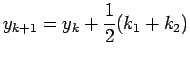
Initial x	Initial y	Stepsize h	Appx. Y	Exa. Y	Error	k1	k2
0.00000	1.00000	0.10000	1.00000	1.00000	0.00000	0.1	0.121
0.1000000	1.00000	0.10000	1.1105	1.11111	0.00061	0.1	0.146531
0.2000000	1.11050	0.10000	1.233765513	1.25000	0.01623	0.123321	0.184168
0.3000000	1.23377	0.10000	1.387510219	1.42857	0.04106	0.152218	0.237076
0.4000000	1.38751	0.10000	1.582157194	1.66667	0.08451	0.192518	0.314947
0.5000000	1.58216	0.1000000	1.835890108	2.00000	0.16411	0.250322	0.006266

			Table 6
Initial x	Initial y	Stepsize h	Appx. Y	Exa. Y	Error	k1	k2
0	1	0.05	1	1	0	0.05	0.055125
0.05	1	0.05	1.0525625	1.052631579	-6.9079E-05	0.055394	0.061378
0.1	1.0525625	0.05	1.110948907	1.111111111	-0.0001622	0.06171	0.068756
0.15	1.110948907	0.05	1.176182339	1.176470588	-0.00028825	0.06917	0.077545
0.2	1.176182339	0.05	1.249540038	1.25	-0.00045996	0.078068	0.088127
0.25	1.249540038	0.05	1.332637341	1.333333333	-0.00069599	0.088796	0.101024
0.3	1.332637341	0.05	1.427547224	1.428571429	-0.0010242	0.101895	0.11696
0.35	1.427547224	0.05	1.536974305	1.538461538	-0.00148723	0.118115	0.136966
0.4	1.536974305	0.05	1.664514529	1.666666667	-0.00215214	0.13853	0.162549
0.45	1.664514529	0.05	1.815054023	1.818181818	-0.0031278	0.164721	0.195975
0.5	1.815054023	0.05	1.995402285	2	-0.00459772	0.199082	0.240788

			Table 7
Initial x	Initial y	Stepsize h	Appx. Y	Exa. Y	Error	k1	k2
0	1	0.025	1	1	0	0.025	0.026266
0.025	1	0.025	1.025625	1.025641026	-1.6026E-05	0.026298	0.027664
0.05	1.025625	0.025	1.051923467	1.052631579	-0.00070811	0.027664	0.029138
0.075	1.051923467	0.025	1.078930846	1.081081081	-0.00215023	0.029102	0.030693
0.1	1.078930846	0.025	1.106685431	1.111111111	-0.00442568	0.030619	0.032337
0.125	1.106685431	0.025	1.135228679	1.142857143	-0.00762846	0.032219	0.034073
0.15	1.135228679	0.025	1.164605572	1.176470588	-0.01186502	0.033908	0.035911
0.175	1.164605572	0.025	1.194865028	1.212121212	-0.01725618	0.035693	0.037857
0.2	1.194865028	0.025	1.226060373	1.25	-0.02393963	0.037581	0.03992
0.225	1.226060373	0.025	1.258249888	1.290322581	-0.03207269	0.03958	0.042109
0.25	1.258249888	0.025	1.291497448	1.333333333	-0.04183589	0.041699	0.044435
0.275	1.291497448	0.025	1.32587326	1.379310345	-0.05343709	0.043948	0.04691
0.3	1.32587326	0.025	1.361454731	1.428571429	-0.0671167	0.046339	0.049547
0.325	1.361454731	0.025	1.398327491	1.481481481	-0.08315399	0.048883	0.05236
0.35	1.398327491	0.025	1.436586603	1.538461538	-0.10187494	0.051595	0.055367
0.375	1.436586603	0.025	1.476338004	1.6	-0.123662	0.054489	0.058586
0.4	1.476338004	0.025	1.517700238	1.666666667	-0.14896643	0.057585	0.062038
0.425	1.517700238	0.025	1.560806538	1.739130435	-0.1783239	0.060903	0.065749
0.45	1.560806538	0.025	1.605807372	1.818181818	-0.21237445	0.064465	0.069745
0.475	1.605807372	0.025	1.652873554	1.904761905	-0.25188835	0.0683	0.074061
0.5	1.652873554	0.025	1.702200096	2	-0.2977999	0.072437	0.078733

FLOWCHART

Remark. The local error in the Algorithm 3.3 is $O(h^5)$. To achieve this error, we are forced to more computation or in other words spend time to compute $k_1,k_2,k_3$ and $k_4$. It all depends on the nature of the function to estimate the time consumed for the computation. The cost we pay for higher accuracy is more computation. Also, to reduce the local error, we need smaller values of the step size h, which again results in large number of computation. Each computation leads to move of rounding errors. In other words, reduction in discretization error may lead to increase in rounding off error. The moral is that the indiscriminate reduction of step-size need not mean more accuracy.