
Next: 3.1 Algorithm: Runge-Kutta Method Up: Main Previous: 2.1 Theorem:
3. Runge-Kutta MethodRunga- Kutta method is a more general and improvised method than that of the Euler's method. It uses, as we shall see, Taylor's expansion of a smooth function.
Before we proceed further, the following questions may arise in our mind, which has not found place in our discussion.
(a) How does one choose the starting values, sometimes called starters that are required to implement an algorithm ?
(b) Is it desirable to change the step size (or the length of the interval) h during the computation if the error estimates demands a change in h?
For the present, the discussion about question (b) is not taken up. We try to look more on question (a) in the ensuing discussion. There are many self-starter methods, like the Euler method which uses the initial condition. But these methods, are normally, not very efficient since the error bounds may not be "good enough". We have seen, in Theorem 2.1 that the local error (neglecting the rounding-off error) isin the Euler's Algorithm. This shows that the smaller the value of h, better the approximations are, But a smaller values of the step size h increases the volume of computations. Moreover the error of order
( h is the step size) may not be sufficiently accurate for many problems. So we look into a few methods where the error is of higher order. They are Runge-Kutta (in short R-K) methods. Let us analyze how the algorithm is reached before we actually state it. We consider the IVP
. Define
for k=0,1,2...n with
and
. We now assume that both y and f are "smooth" functions ( thereby we mean that the derivatives, could be partial also exists and are continuous upto certain "desired" order). Using Taylor's series, we now have
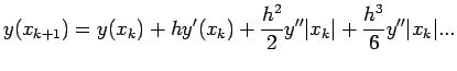 |
(3.1) |
(
denotes the approximate value of y at
, to be defined shortly.) Consider, for k=0,1,2..n-1
| (3.2) |
where
| (3.3) |
and
| (3.4) |
where p,q,
and
are constants. When
, (3.2) reduces to the Euler Algorithm. We choose p,q,
). From the definition of
we have
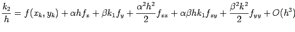
where
,
, .... denotes the partial derivatives of f w.r.t. x,y, .... respectively. Substituting these values in (3.2), we have
 |
(3.5) |
A comparison of (3.1) and (3.4), leads to the choice
| (3.6) |
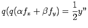 |
(3.7) |
in order that the powers of h upto
match (in some sense) in the approximate values of
. Here we note that
Now we choose
,p and q so that (3.6) and(3.7) are satisfied. One of the simplest solution is
 and
and Thus, we are lead to define
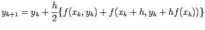 |
(3.8) |
Evaluation of
A few things are worthwhile to be noted in the above discussion. Firstly, we need the existence of partial derivatives of f upto 3 third order for R-K method of order 2. For higher order methods, we need f to be more smooth. Secondly we note that the local truncation error( in R-K method of order 2) is of the order
. Again, we remind the readers here that the round off error in the case of implementation has not been considered. Also in (3.8), the partial derivatives of f do not appear. In short, we are likely to get a better accuracy in Runge-Kutta method of order 2 in comparison with the Euler's method. Formally, we state the Runge-Kutta method of order 2.

Next: 3.1 Algorithm: Runge-Kutta Method Up: Main Previous: 2.1 Theorem: