
![]()
![]()
Next: Sample Programs Up:Main Previous:Hyperbolic Equation
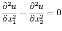
Elliptic equations in two dimensions:
Suppose that R is a bounded region in the
![]() plane with boundary
plane with boundary
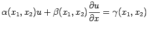
![]() . The equation
. The equation
 |
(30) |
| (31) |
 |
(32) |
 |
(33) |
 |
(34) |
subject to
![]() on the boundary of the unit square
on the boundary of the unit square
![]() . The square region is covered by a grid with sides parallel to the coordinate axes and the grid spacing is
. The square region is covered by a grid with sides parallel to the coordinate axes and the grid spacing is ![]() . If
. If ![]() , the number of internal grid points or nodes is
, the number of internal grid points or nodes is ![]() . The coordinates of a typical internal grid point are
. The coordinates of a typical internal grid point are ![]() ,
, ![]() (
( ![]() and m integers ) and the value of
and m integers ) and the value of ![]() at this grid point is denoted by
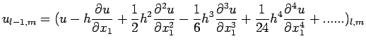
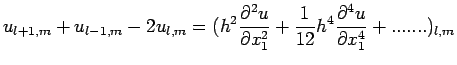
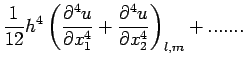
at this grid point is denoted by ![]() . Using Taylor's Theorem, we obtain
. Using Taylor's Theorem, we obtain
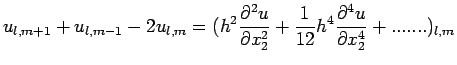
![$\displaystyle u_{l+1,m}+u_{l-1,m}+u_{l,m+1}+u_{l,m-1}-4u_{l,m}=
\left[ h^{2}\le...
..._{1}^{4}}+\frac{\partial^{ 4}u}{\partial x_{2}^{
4}}\right)+......\right]_{l,m}$](img319.png)
| (35) |
| (36) |
where ![]() is a matrix of order
is a matrix of order ![]() given by
given by
with ![]() the unit matrix of order
the unit matrix of order ![]() and
and ![]() a matrix of order
a matrix of order
![]() given by
given by
B
= 
The vectors ![]() and
and ![]() are given by
are given by
U=
![]()
respectively, where ![]() denotes the transpose. The elements of the vector U constitute the
denotes the transpose. The elements of the vector U constitute the ![]() unknowns
unknowns
![]() and the elements of the vector K depend on the boundary values
and the elements of the vector K depend on the boundary values
![]() at the grid points on the perimeter of the unit square. Because of the large number of zero element in the matrix A, iterative methods are often used to solve the system (36).
at the grid points on the perimeter of the unit square. Because of the large number of zero element in the matrix A, iterative methods are often used to solve the system (36).
![]()
![]()
Next: Sample Programs Up:Main Previous:Hyperbolic Equation