: この文書について...
: lec1
: Numerical Differentiation:
The problem of numerical
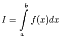
integration is that of determining an approximate value of the
integral
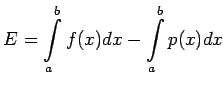
If  is the interpolating polynomial of degree n which
approximate
is the interpolating polynomial of degree n which
approximate  on
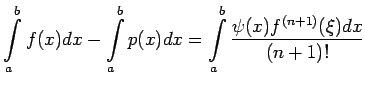
on ![$ [a,b]$](img493.png) then for the error
we have the following theorem:
then for the error
we have the following theorem:
Theorem: Let
 be
be  points on
the interval . Let
points on
the interval . Let  be the corresponding values of
 at
at  . Let be the polynomial of degree n which
interpolates at the n+1 points
. Let be the polynomial of degree n which
interpolates at the n+1 points
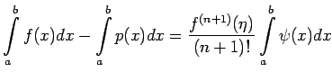
 Then if
does not change sign on the interval , the error of
numerical integration is given by
For some point
Then if
does not change sign on the interval , the error of
numerical integration is given by
For some point  in .
in .
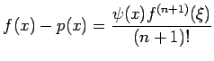
Proof: We have from the error formula for the
interpolation polynomial
Integration, we get
If  does not change sign on the interval , then we
can apply the second mean value theorem of integral calculus, we
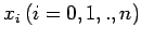
obtain the desired result. Let us assume that the function
can be computed at a set of n+1 equally spaced points
does not change sign on the interval , then we
can apply the second mean value theorem of integral calculus, we
obtain the desired result. Let us assume that the function
can be computed at a set of n+1 equally spaced points
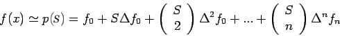
 . Then can be approximated by the Newton
forward difference interpolating polynomial
where
. Then can be approximated by the Newton
forward difference interpolating polynomial
where
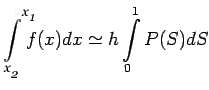
 . Thus we have
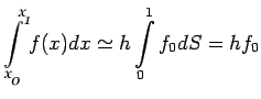
Let us take n=0, we get
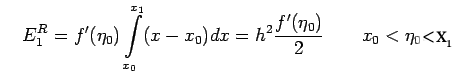
This is known as rectangular rule and we denote it as
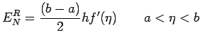
The error of this approximation is
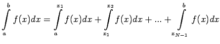
To find the integral of f(x) over an extended interval we
subdivide into N equal subdivision, setting
. Thus we have
Let us take n=0, we get
This is known as rectangular rule and we denote it as
The error of this approximation is
To find the integral of f(x) over an extended interval we
subdivide into N equal subdivision, setting
 Now
Applying the above formula to each integral of yields the
rectangular rule for the integral of over an interval
:
and the error is given by
and if
Now
Applying the above formula to each integral of yields the
rectangular rule for the integral of over an interval
:
and the error is given by
and if  is continuous over
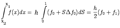
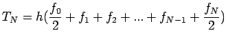
A more accruable formula can be obtained by taking n=1, and we
find that
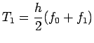
which is known as Trapezoidal rule denoted by
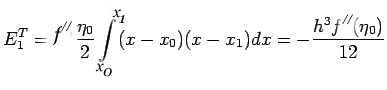
with the error given by
To obtain the integral over the interval , we subdivide
into N equal parts and use the above formula to each
integral, this yields
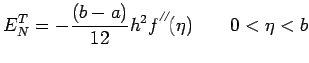
The error of this formula is given by
Simpson's Rule
is continuous over
A more accruable formula can be obtained by taking n=1, and we
find that
which is known as Trapezoidal rule denoted by
with the error given by
To obtain the integral over the interval , we subdivide
into N equal parts and use the above formula to each
integral, this yields
The error of this formula is given by
Simpson's Rule
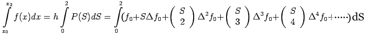
We integrate over the double interval
![$ [x_0, x_2]$](img523.png) of width
of width
 and get
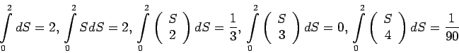
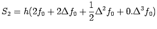
By direct integration, we find that
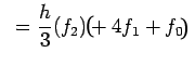
If we retain difference through the third
order, we obtain an approximation
This formula is called Simpson's rule.
and get
By direct integration, we find that
If we retain difference through the third
order, we obtain an approximation
This formula is called Simpson's rule.
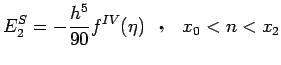
The error of this formula is given by
To extend Simpson's rule in integration over an interval ,
we now divide into an even number 2N of sub intervals of
width h so that
and
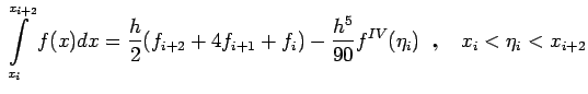
Using Simpson's rule over
the interval
![$ [x_i,x_{i+2}]\,(i=0,2,...,2N-2)$](img532.png) ,we have
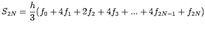
If we now sum over the N subgroups of the intervals each, we
obtain
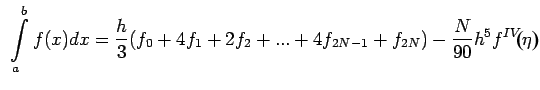
and using Simpson's rule for integration over an interval
which has been subdivided into 2N subintervals of length h is
and since
,we have
If we now sum over the N subgroups of the intervals each, we
obtain
and using Simpson's rule for integration over an interval
which has been subdivided into 2N subintervals of length h is
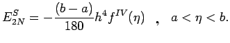
and since
 , the error term is
: この文書について...
: lec1
: Numerical Differentiation:
root
平成18年1月24日
![$\displaystyle E^R_N=\frac{ h^2}{2}[f'(\eta_0)+f'(\eta_1)+...+f'(\eta_{N-1})]$](img515.png)