Gaussian Elimination

To solve $Ax=b$, we reduce it to an equivalent system $Ux=g$, in which U is upper triangular. This system can be easily solved by a process of backward substitutions.
Denote the original linear system by $A^{(1)}x=b^{(1)}$, where $A^{(1)}=[a^{(1)}_{ij}],\,\, b^{(1)}=[b_1^{(1)},...b_n^{(1)}]^T \,\,\, 1\leq i , j\leq n$ and n is the order of the system. We reduce the system to the triangular form $Ux=g$ by adding multiples of one equation to another equation, eliminating some unknown from the second equation. Additional row operations are used in the modifications given later. We define the algorithm in the following. Gaussian elimination algorithm:
Step 1: Assume $a_{11}^{(1)}$. Define the row multipliers by

$$m_{i1}=\frac{a_{i1}^{(1)}}{a_{11}^{(1)}} \,\,\,\, i=2,3,...,n$$

These are used in eliminating the $x_1$ term form equation 2 through n. Define

$$a_{ij}^{(2)}=a_{ij}^{(1)}-m_{i1}a_{1}^{(1j)}\,\,\,\,\,\, i,j=2,...,n$$

$$b_{i}^{(2)}=b_{i}^{(1)}-m_{i1}b_{1}^{(1)} \,\,\,\,\,\, i=2,...,n$$

Also, the first rows of A and B are left undisturbed, and the first column of $A^{(1)}$, below the diagonal, is set to zero. The system $A^{(2)}x=b^{(2)}$ looks like

$$\left[% \begin{array}{ccccc} a_{11}^{(1)} & a_{12}^{(1)} &... ...} \\ . \\ . \\ b_{n}^{(2)} \\ \end{array}% \right]$$

We continue to eliminate unknowns, going onto columns 2, 3, etc., and this is expressed generally as follows.
Step k: Let $1 \leq k \leq n-1$. Assume that $A^{(k)}x=b^{(k)}$ has been constructed with $x_1,x_2,...x_{k-1}$ eliminated as successive stages and $A^{(k)}$ has the form

$$A^{(k)}=\left[% \begin{array}{cccccccc} a_{11}^{(1)} & a_{... ..._{nk}^{(k)} & . & . & a_{nn}^{(k)} \\ \end{array}% \right]$$

Assume $a_{kk}^{(k)}\neq 0$. Define the multipliers.

$$m_{ik}=\frac{a_{ik}^{(k)}}{a_{kk}^{(k)}} \qquad\qquad i=k+1, ...,n$$ (1)

Use these to remove the unknown's $x_k$ from equations K+1 through n. Define

$$a_{ij}^{(k+1)}=a_{ij}^{(k)}-m_{ik}a_{kj}^{(k)}$$ (2)

$$b_i^{(k+1)}=b_i^{(k)}-m_{ik}b_k^{(k)} \,\,\,\,\,\,L i,j=k+1,...,n$$

The earlier rows 1 through K are left undisturbed, and zeros are introduced into column K below the diagonal element. By continuing in this manner, after n-1 steps we obtain $A^{(n)} x=b^{(n)}$ i.e

$$\left[% \begin{array}{ccccc} a_{11}^{(1)} & . & . & . & a_... ... . \\ . \\ . \\ b_{n}^{(n)} \\ \end{array}% \right]$$

Let $U=A^{(n)}$ and $g=b^{(n)}$. The system Ux=g is upper triangular and easy to solve by back substitution; i.e

$$x_n=\frac{g_n}{u_{nn}}$$

and

$$x_k=\frac{1}{u_{kk}}[g_k- \sum\limits_{j=k+1}^n u_{kj}x_j]\,\,\,\ , \, k=n-1,n-2, ...1$$

This completes the Gaussian elimination algorithm.
Example: solve the linear system

$$x_1+2x_2+x_3=0$$

$$2x_1+2x_2+3x_3=3$$

$$-x_1-3x_2 \qquad\; =2$$

Represent the linear system by the augmented matrix

$$[A/b]=\left[% \begin{array}{ccc\vert c} 1 & 2 & 1 &0\\ 2 & 2 & 3 &3\\ -1 & -3&0 & 2 \\ \end{array}% \right]$$

and carry out the row operations as given below

$$\left[% \begin{array}{ccc\vert c} 1 & 2 & 1 & 0 \\ 2 & ... ... & 3 \\ 0 & 0 & 1/2 & 1/2 \\ \end{array}% \right]=[U/g]$$

Solving Ux=g, We get

$$x_3=1, \,\,\, x_2=-1,\,\,\, x_1=1$$

Triangular factorization of a matrix
Denote by L the lower triangular matrix given by

$$L=\left[% \begin{array}{cccccc} 1 & 0 & 0 & . & . & 0 \\ ... ...\ m_{n1} & m_{n2} & . & . & . & 1 \\ \end{array}% \right]$$

Theorem: If L and U are the lower and upper triangular Matrices as defined above, then

$$A=LU$$

Proof: The proof is an algebraic manipulation, making use of (1) and (2) as given above. We write

$$(LU)_{ij}=[m_{i1},...m_{i,i-1},1,0,..0]\left[% \begin{array}... ...{ij} \\ 0 \\ . \\ . \\ 0 \\ \end{array}% \right]$$

For $i \leq j,$

$$(LU)_{ij}=m_{i1}u_{1j}+m_{i2}u_{2j}+...+m_{i,i-1}u_{i-1,j}+u_{ij}$$

$$=\sum\limits_{k=1}^{i-1}m_{ik}a_{kj}^{(k)}+a_{ij}^{(i)}$$

$$=\sum\limits_{k=1}^{i-1}[a_{ij}^{(k)}-a_{ij}^{(k=1)}]+a_{ij}^{(i)}$$

$$=a_{ij}^{(1)}=a_{ij}$$

This completes the proof.
Corollary: With the matrices A, L and U as in the above theorem.

$$det(A)=u_{11}\,u_{22}...u_{nn}$$

$$=a_{11}^{(1)}a_{22}^{(2)}...a_{nn}^{(n)}$$

Proof: Follows by the product rule for determinants

$$det(A)=det(L)det(U)$$

Since L and U are triangular, their determinants are the product of their diagonal elements. The desired result follows easily, since det(L)=1.
Example: For the system of the previous example

$$L= \left[% \begin{array}{ccc} 1 & 0 & 0 \\ 2 & 1 & 0 \... ...\\ 0 & -2 & 1 \\ 0 & 0 & 1/2 \\ \end{array}% \right]$$

It is easy to see that A=L U. Also det(A)=det(U)=-1
Pivoting and Scaling in Gaussian Elimination
At each stage of the elimination process given above, we assumed the appropriate pivot element $a_{kk}^{(k)}\neq 0$. To remove this assumption, begin each step of the elimination process by switching rows to put a non zero element in the pivot position. If none such exists, then the matrix must be singular, contrary to assumption.
It is not enough, however, to just ask that pivot element be nonzero. Nonzero but very small pivot element will yield gross errors in further calculation and to guard against this and propagation of rounding errors, we introduce pivoting strategies.
Definition: (Partial Pivoting). For $1 \leq k \leq n-1$ in the Gaussian elimination process at stage k, let

$$C_k=\max\limits_{k\leq i \leq n} \vert a_{ik}^{(k)}\vert$$

Let i be the smallest row index, $i\geq k$, for which the maximum $C_k$ is attained. If $i > k,$ then switch rows k and i in A and b, and proceed with step k of the elimination process. All the multipliers will now satisfy

$$\vert m_{ik}\vert\leq 1 \qquad \quad i=k+1,..., n$$

This helps in presenting the growth of elements in $A^{(k)}$ of greatly varying size, and how this lessens the possibility for large loss of significance errors.
Definition: (Complete Pivoting). Define

$$C_k=\max\limits_{k \leq i, \, j \leq n} \vert a_{ij}^{(k)}\vert$$

Switch rows of A and b and columns of A to bring to the pivot position an element giving the maximum $C_k$.
However, complete pivoting is more expansion and thus partial pivoting is more often used
Example: Consider solving the system with and without pivoting:

$$.729x+.81y+.9z=.6867$$

$$x+y+z=.8338$$

$$1.331x+1.21y+1.1z=1.000$$

The exact solution rounded to four significant digits is

$$x=.2245 \qquad y=.2814 \qquad z=.3279$$

1. Solution without pivoting: Using four decimal arithmetic

$$\left[% \begin{array}{ccc\vert c} .7290 & .8100 & .9000 & ... ... \\ 1.331 & 1.210 & 1.100 & 1.000 \\ \end{array}% \right]$$

$$m_{31}=1.826\big{\downarrow} m_{21}=1.372$$

$$\left[% \begin{array}{ccc\vert c} .7290 & .8100 & .9000 & ... ...\\ 0.0 & -.2690 & -.5430 & -.2540 \\ \end{array}% \right]$$

$$\big{\downarrow} m_{32}=2.423$$

$$\left[% \begin{array}{ccc\vert c} .7290 & .8100 & .9000 & ... ...4 \\ 0.0 & 0.0 & .02640 & .008700 \\ \end{array}% \right]$$

The solution is

$$x=.2251 \qquad y=.2790 \qquad z= .3295$$

2. Solution with pivoting: To indicate the interchange of rows i and j, we will use the notation $r_i\leftrightarrow r_j$

$$\left[% \begin{array}{ccc\vert c} .7290 & .8100 & .9000 & ... ... \\ 1.331 & 1.210 & 1.100 & 1.000 \\ \end{array}% \right]$$

The solution is

$$x=.2246\quad y=.2812 \quad z=.3280$$

The error in (3) is form seven to sixteen times larger them it is for (4), depending upon the component of the solution being considered. The results in (4) have one more significant digit than those in (3). This illustrates the positive effect that the use of pivoting can have on the error for Gaussian elimination.
Scaling: It has been observed that if the elements of the coefficient matrix A vary greatly in size, then it is likely that large loss of significance errors will be introduced and the propagation of sounding errors will be worse. To avoid this problem, we usually scale the matrix A so that the elements vary less. This is usually done by multiplying the rows and columns by suitable constants. If we let B denote the result of row and column scaling in A, then

$$B=D_1 AD_2$$

Where $D_1$ and $D_2$ are the diagonal matrices, with .......... scaling constants. To solve $Ax=b$, observe that

$$D_1AD_2(D_2^{-1}x)=D_1b$$

Thus we solve for x by solving

$$Bz=D_1b \qquad x=D_2 z$$

Restricting ourselves to row scaling, we attempt to choose the coefficients so as to have

$$\max\limits_{1 \leq j \leq n}\vert b_{ij}\vert =1 \qquad i=1,...,n$$

where $B=[b_{ij}]$ is the result of scaling A.
Gauss-Jordan Method This procedure is much the same as Gauss elimination including the possible use of pivoting and scaling. It differs in eliminating the unknown in equation above the diagonal as well as below it. In step K of the elimination, choose the pivot element as before. Then define

$$a_{kj}^{(k+1)}=\frac{a_{kj}^{(k)}}{a_{kk}^{(k)}} \qquad j=k,...n$$

$$b_k^{k+1}=\frac{b_k^{(k)}}{a_{kk}^{(k)}}$$

Eliminate the unknown $x_k$ in equation both above and below equation K. Define

$$a_{ij}^{(k+1)}=a_{ij}^{(k)}-a_{ik}^{(k+1)} \qquad j=k,...n$$

$$b_{i}^{(k+1)}=b_{i}^{(k)}-a_{ij}^{(k)} \qquad i=1,...,n, \quad i\neq k$$

The procedure will correct the augmented matrix $[A/b]$ to $[I/b^{(b)}]$, so that the solution is $x=b^{(n)}$.
The choleski Method
Let A be a symmetric and positive definite matrix of order n. The matrix is positive definite if $(Ax,x)=\sum\limits_{i=1}^n\sum\limits_{j=1}^n a_{ij}x_ix_j > 0$    for all $x \epsilon R^n,\, x \neq 0$, for such a matrix A, there is a very convenient factorization and can be carried out without any need for pivoting or scaling. This is called choleski factorization and that is we can find a lower triangular real matrix L such that

$$A=LL^T$$

Construction of the matrix L: Let $L=(l_{ij})$ with $l_{ij}=0$ for $j> i$. Begin the construction of L by multiplying the first row of A times the first column of $L^T$, we get

$$l^2_{11}=a_{11}$$

Because A is positive definite, $a_{11} >0$ and $l_{11}=\sqrt{a_{11}}$. Next, multiply the second row of L times the first two columns of $L^T$ to get

$$l_{21}l_{11}=a_{21} \qquad \qquad l^2_{21}+l^2_{22}=a_{22}$$

Again, we can solve for the unknowns $l_{21}$ and $l_{22}$. In general for $i=1,2,...,n,$

$$l_{ij}=\frac{a_{ij}-\sum\limits_{k=1}^{j-1}l_{ik}l_{jk}}{l_{jj}} \qquad \qquad j=1,...i-1$$

$$l_{ii}=[a_{ii}-\sum\limits_{k=1}^{i-1}l^2_{ik}]^{1/2}$$ (5)

The square root in (5) of choleski's method can be avoided by using a slight modification of the factorization. That is to find a diagonal matrix D and a lower triangular matrix $\hat{L}$, with unity on the diagonal, such that

$$A=\hat{L}D\hat{L}^T$$ (6)

Example: Consider the Hilbert matrix of order 3,

$$A=\left[% \begin{array}{ccc} 1 & 1/2 & 1/3 \\ 1/2 & 1/3 & 1/4 \\ 1/3 & 1/4 & 1/5 \\ \end{array}% \right]$$

For the choleski decomposition

$$L=\left[% \begin{array}{ccc} 1 & 0 & 0 \\ 1/2 & 1/2\s... ... 1/3 & 1/2\sqrt{3} & 1/6\sqrt{5} \\ \end{array}% \right]$$

And for (6), we have

$$\hat{L}=\left[% \begin{array}{ccc} 1 & 0 & 0 \\ 1/2 & 1... ... 0 & 1/12 & 0 \\ 0 & 0 & 1/180 \\ \end{array}% \right]$$

Tridiagonal systems
The matrix $A=[a_{ij}]$ is tridiagonal, if $a_{ij}=0$ for $\vert i-j\vert>1$
Let

$$A=\left[% \begin{array}{ccccccc} a_1 & c_1 & 0 & 0 & . & .... ...b_n & a_n \\ \end{array}% \right],\mbox{ with } det(A)\neq 0$$

Consider $A=LU$

$$=\left[% \begin{array}{cccccc} \alpha_1 & 0 & . & . & . & ... ... & 1 & r_{n-1} \\ & & & & 0 & 1 \\ \end{array}% \right]$$

The elements $\alpha_i's$ and $r_i's$ can be computed recursively as:

$$a_1=\alpha_1 \qquad \qquad a_1r_1=c_1$$

$$a_i=\alpha_i+b_i.r_{i-1} \qquad i=2,...,n$$

$$\alpha_ir_i=c_i \qquad i=2,3,...,n-1$$

These can be solved to give

$$\alpha_1=a_1 \qquad r_1=c_1/\alpha_1$$

$$\alpha_i=a_i-b_ir_{i-1} \qquad r_i=c_i/\alpha_i \qquad i=2,3,...,n-1; \,\, \alpha_i \neq 0 (\because$$   A is nf$$)$$

$$\alpha_n=a_n-b_nr_{n-1}$$

To solve $LUx=f$, let $Ux=z$ and $Lz=f$. Then

$$z_1=f_1/\alpha_1 \qquad z_i=\frac{f_i-b_iz_{i-1}}{\alpha_i} \qquad i=2,3,...$$

$$x_n=z_n \qquad x_i=z_i-r_ix_{i+1}\qquad i=n-1,n-2,...,1$$

Error Analysis:
Consider solving the system $Ax=b$, Where A is a non-singular matrix of order n. Denote by $x_t$ and $x_c$ the true and computed solutions, respectively, of $Ax=b$. One possible measure of the error in the computed solution would be the magnitude of the residual vector.

$$r=Ax_c-b$$

If

$$r^T=(r_1,r_2,...,r_n),$$   then$$\vert r\vert=(\sum\limits_{i=1}^nr^2_i)^{1/2}.$$

Remarks:
But this is not appropriate of error analysis as $\vert r\vert$ can be quite small even though $x_c$ is a very erroneous solution. This can be justified in the following manner: if $A^{-1}$ has some large elements, then r may be very small even if $x_c$ is substantially different from the true solution. For

$$r=A(x_c-x_t)$$

or

$$x_c-x_t=A^{-1}r$$

Therefore, if some elements of $A^{-1}$ are large, a small component of r can still mean a large difference between $x_c$ and $x_t$, or conversely, $x_c$ may be far from $x_t$ but r can nevertheless still be small. In other words, an accurate solution (i.e a small difference between $x_c$ and $x_t$) will always produce small residuals but small residuals do not guarantee an accurate solution.
If the system $Ax=b$ is such that $A^{-1}$ contains some very large elements, then we try the matrix and, therefore, the system of equations is ill-conditioned. The following simple example will illustrate the dangers inherent in solving ill-conditional system. Consider the system

$$2x+6y = 8$$

$$2x+6.000014 = 8.00001$$ (7)

Which has the solution x=1, y=1, and the system

$$2x+6y = 8$$

$$2x +5.99999y =8.00002$$ (8)

which has the solution x=10, y=-2. Here a change of .00002 in $a_{22}$ and .00001 in $b_2$ has caused a gross change in the solution. The inverse of the matrix of coefficients in (7) has elements whose order of magnitude is $10^5$, which indicates the ill conditioning of A.
A more reasonable measure of the error is given by

$$E=\vert x_c-x_t\vert$$

It is this error we shall try to estimate here. Any bound on E will depend on the magnitude of the round off errors incurred, the order of the matrix A, and the size of $A^{-1}$. One approach to finding such a bound would be to consider the worst possible case of round off as each stage of the method and to desire a bound based on the accumulation of these errors. Since the round off at one stage is quite complicated function of the round off at precious stages, more bounds are difficult to calculate. Instead our approach here will be to estimate the perturbed system of equations whose true solution is the calculated solution $x_c$. That is, the completed solution $x_c$ is the true solution of some system which we write as

$$(A+\delta A)x = b+\delta b$$

We can not hope to find $\delta A$ and $\delta B$ precisely; our object is to find bounds on their elements.
We have

$$x_c-c_t=(A+\delta A)^{-1}(b+\delta b)-A^{-1}b$$

$$\qquad=[(A+\delta A)^{-1}-A^{-1}]b+(A+\delta A)^{-1}\delta b$$

$$\qquad=[(A+\delta A)^{-1}-A^{-1}]b+(I+A^{-1}\delta A)^{-1}A^{-1}\delta b$$ (9)

In order to find a bound E, we consider the following two Norm of the matrix A.
i) Euclidean Norm of A is defined as

$$\vert\vert A\vert\vert _E=(\sum\limits_{i=1}^m\sum\limits_{j=1}^na^2_{ij})^{1/2}$$

ii) Spectral Norm of A is defined as

$$\vert\vert A\vert\vert _s=\max\limits_i[\lambda _i(AA^T)]^{1/2}$$

Where the notation $\lambda_i(AA^T)$ denotes an eigen value of $AA^T$. Both of these norms are defined for any m x n matrix. For vectors we define the norm in the Enclidean reverse norm $\vert\vert x\vert\vert=(x^Tx)^{1/2}$.
The Enclidean norm may also be expressed as

$$\vert\vert A\vert\vert _E=[tr(AA^T)]^{1/2}$$

Where tr denotes the trace. Since the trace of a matrix is the sum of its eigen values $\vert\vert A\vert\vert^2_E=\sum\limits_{i=1}^n\lambda _i(AA^T)$ where n is the order of $AA^T$
Thus we have the important result

$$\vert\vert A\vert\vert _s\leq \vert\vert A\vert\vert _E$$

For our purpose the spectral norm is much more useful of the two norms. We shall here after drop the subscript s on the spectral norm. We also need to use the spectral radius, which is defined as $P(A)=\max\limits_i \vert\lambda_i(A)\vert$, Thus $\vert\vert A\vert\vert=[p(AA^T)]^{1/2}$ , and when A is symmetric, we have $\vert\vert A\vert\vert=p(A)$
We need the following theorem to obtain the error bound.
Theorem: Let A be a square matrix and x any vector. Then

$$\max\limits_x\frac{\vert\vert Ax\vert\vert}{\vert\vert x\vert\vert}=\vert\vert A\vert\vert$$

Proof: Let $\lambda_1$ be the largest eigen value in magnitude of $AA^T$. For any x

$$\frac{\vert\vert Ax\vert\vert^2}{\vert\vert x\vert\vert}-\vert\ve... ...rt^2=\frac{x^TA^TAx}{x^Tx}-\lambda_1=\frac{x^T(A^TA-\lambda_1I)x}{x^Tx}\leq 0,$$

Since the eigen value of $A^TA-\lambda_1I$ are nonpositive and therefore the numerator is negative semi-definite. Equality holds when x is or eigen vector of $A^TA$ corresponding to $\lambda_1$. Hence the theorem.
Corollary 1. $\vert\vert A\vert\vert \geq \rho (A)$
Proof: The result follows by letting x be the eigen vector corresponding to any eigen value of A.
Corollary 2. If $\vert\vert A\vert\vert < 1$, then I+A is non-singular.
Proof: $\lambda _i(I+A)=1+\lambda_i(A)$ ($\because$ the eigen values of I are 1.) Thus $\vert\lambda_i(I+A)\vert\geq 1-\vert\lambda_i(A)\vert\geq 1-\vert\vert A\vert\vert> 0$
Corollary 3. If $\vert\vert A\vert\vert < 1$,then

$$\vert\vert(I+A)^{-1}\vert\vert\leq \frac{ 1}{1-\vert\vert A\vert\vert}$$

and

$$\vert\vert(I+A)^{-1}-I\vert\vert\leq \frac{\vert\vert A\vert\vert}{1-\vert\vert A\vert\vert}$$

Proof: Since (I+A) is non-singular by corollary 2, we have

$$I=(I+A)^{-1}(I+A)=R+RA,$$   where$$R=(I+A)^{-1}$$

Taking norm, we have

$$1=\vert\vert I\vert\vert \geq \vert\vert R\vert\vert -\vert\vert ... ...t \geq \vert\vert R\vert\vert -\vert\vert R\vert\vert \, \vert\vert A\vert\vert$$

From which it follows that

$$\vert\vert R\vert\vert=\vert\vert(I+A)^{-1}\vert\vert \leq \frac{1}{1-\vert\vert A\vert\vert}$$

The second part also follows easily.
Corollary 4. If A is non-singular and $\vert\vert A^{-1}B\vert\vert<1$, then A+B is nonsingular and

$$\vert\vert(A+B)^{-1})-A^{-1}\vert\vert\leq k\, \vert\vert A^{-1}\vert\vert$$

Where $K=\vert\vert A^{-1}B\vert\vert/(1-\vert\vert A^{-1}B\vert\vert)$
Proof: Using corollary 2, the non-singularity of both A+B and $I +A^{-1}B$ follows since
$A+B =A(I+A^{-1}B)$. We have
$(A+B)^{-1}=(I+A^{-1}B)^{-1}A^{-1}$ Thus

$$(A+B)^{-1}-A^{-1}=[(I+A^{-1}B)^{-1}-I]A^{-1}$$

Taking norm, we have

$$\vert\vert(A+B)^{-1}-A^{-1}\vert\vert\leq \vert\vert(I+A^{-1}B)^{... ...A^{-1}B\vert\vert}{1-\vert\vert A^{-1}B\vert\vert}.\vert\vert A^{-1}\vert\vert;$$

With the definition of vector norm given earlier. We see that

$$E=x_c-x_t$$

Using corollaries 3 and 4, we have from (9),

$$\vert\vert x_c-x_t\vert\vert\leq \vert\vert(A+\delta A)^{-1}-A^{-... ...a A)^{-1}\vert\vert \,\vert\vert A^{-1}\vert\vert\,\vert\vert\delta b\vert\vert$$

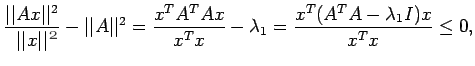
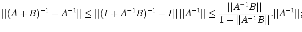
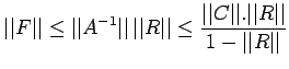
$$\leq \frac{\vert\vert A^{-1}\vert\vert}{1-\vert\vert A^{-1}\vert\... ...ert\vert A^{-1}\vert\vert\,\vert\vert b\vert\vert+\vert\vert\delta b\vert\vert]$$ (10)

Where we have assumed that $\vert\vert A^{-1}\vert\vert\,\vert\vert\delta A\vert\vert< 1$. One can see that bound (iv) depends upon bounds on $\vert\vert\delta A \vert\vert$ and $\vert\vert\delta b\vert\vert$ in addition to a bound on $\vert\vert A^{-1}\vert\vert$.
A priori Error Estimate
In solving the system

$$Ax=b$$ (11)

by any procedure, round off errors will in general be introduced. But if the problem is well posed these errors can be kept with in reasonable bounds. By a problem to be well posed, we mean that 'small' changes in the data lead to 'small' changes in the solution.
Suppose that the matrix A and b in (11) are perturbed by the qualities $\delta A$ and $\delta b$. Then if the perturbation in the solution x of (11) is $\delta x$, we have

$$(A+\delta A((x+\delta n)= b+\delta b$$ (12)

Now an estimate of the relative change in the solution can be given in terms of the relative changes in A and b by means of the following.
Theorem: Let A be non-singular and the perturbation $\delta A$ be so small that

$$\vert\vert\delta A\vert\vert< \frac{1 }{\vert\vert A^{-1}\vert\vert}$$ (13)

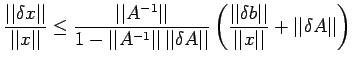
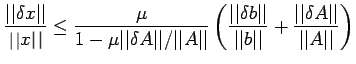
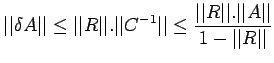
Then if x and $\delta x$ satisfy (11) and (12), we have

$$\frac{\vert\vert\delta x\vert\vert}{x}\leq \frac{\mu}{1-\mu\vert\... ...b\vert\vert}+\frac{\vert\vert\delta A\vert\vert}{\vert\vert A\vert\vert}\right)$$

Where the condition number $\mu$ is defined as

$$\mu=\mu (A)\equiv \vert\vert A^{-1}\vert\vert.\vert\vert A\vert\vert$$ (14)

Proof: Since $\vert\vert A^{-1}\delta A\vert\vert\leq \vert\vert A^{-1}\vert\vert\,\vert\vert\delta A\vert\vert < 1$ by (13), it follows that by corollary 2 and 3, the matrix $I + A^{-1}\delta A$ is non singular and further that

$$\vert\vert(I+A^{-1}\delta A)^{-1}\vert\vert\leq \frac{ 1}{1-\vert... ...ert}\leq \frac{1}{1-\vert\vert A^{-1}\vert\vert\,.\vert\vert\delta A\vert\vert}$$

Now multiply (12) $A^{-1}$, using (11) and solving for $\delta x$, we get

$$\delta x=(I+A^{-1}\delta A)^{-1}A^{-1}(\delta b-\delta Ax)$$

Taking norm and divide by $\vert\vert x\vert\vert$ we get

$$\frac{\vert\vert\delta x\vert\vert}{\vert\vert x\vert\vert}\leq \... ...\delta b\vert\vert}{\vert\vert x\vert\vert}+\vert\vert\delta A\vert\vert\right)$$

Now form (11) it is clean that $\vert\vert x\vert\vert\geq \vert\vert b\vert\vert/\vert\vert A\vert\vert;$ this gives

$$\frac{\vert\vert\delta x\vert\vert}{\vert\vert x\vert\vert}\leq \... ...b\vert\vert}+\frac{\vert\vert\delta A\vert\vert}{\vert\vert A\vert\vert}\right]$$ (15)

which yields the result using the definition (14).
The estimate (15) shows that small relative change in b and A cause small relative changes in the solution if the factor

$$\frac{\mu}{1-\mu\vert\vert\delta A\vert\vert/\vert\vert A\vert\vert}$$

is not too large. The condition (13) is equivalent to $\mu\frac{\vert\vert\delta A\vert\vert}{\vert\vert A\vert\vert} < 1$. Thus, it is clear that when the condition number $\mu A$ is not too large, the system (11) is well conditioned. Note that we can not expect $\mu A$ to be small compared to unity ... .

$$\vert\vert I\vert\vert=\vert\vert A^{-1}A\vert\vert\leq \mu (A)$$

A Posteriori Error Estimate
Although we do not advocate inverting a matrix to solve linear system, it is of interest to consider error estimates related to computed inverses. Let A be the matrix to be inverted and let C be the computed inverse. The error in the inverse is defined by

$$F=C-A^{-1}$$ (16)

We also use another measure of error called the residual matrix:

$$R=I-CA$$ (17)

We have the following result.
Theorem: If $\vert\vert R\vert\vert < 1$, then A and C are non-singular, and

$$\vert\vert A^{-1}\vert\vert\leq \vert\vert c\vert\vert/q-\vert\vert R\vert\vert$$

$$\vert\vert F\vert\vert \leq \vert\vert c\vert\vert.\vert\vert R\vert\vert/(1-\vert\vert R\vert\vert)$$

Proof: Since $\vert\vert R\vert\vert < 1$, I-R is non-singular(by an earlier theorem) and

$$\vert\vert(I-R)^{-1}\leq \frac{1}{1-\vert\vert R\vert\vert}$$

Now $I-R=CA$

$$0 \neq det (I-R)=det(CA)=det (c) det (A)$$

and thus both det(c) and det(A) are non zero. This proves that both A and C are non singular. Now $A^{-1}C^{-1}=(I-R)^{-1}$ or

$$A^{-1}=(I_R)^{-1}C$$

and

$$\vert\vert A^{-1}\vert\vert\leq \vert\vert(I-R)^{-1}\vert\vert\,\vert\vert C\vert\vert\leq\frac{\vert\vert C\vert\vert}{1-\vert\vert R\vert\vert}$$

Also

$$F=-A^{-1}R$$

and

$$\vert\vert F\vert\vert\leq\vert\vert A^{-1}\vert\vert\,\vert\vert... ... \frac{\vert\vert C\vert\vert.\vert\vert R\vert\vert}{1-\vert\vert R\vert\vert}$$

Corollary:
If is of interest to note that with C an approximate inverse of A, we can find the perturbation $\delta A$ so that C is the exact inverse of $A+ \delta A$. That is,

$$C(A+\delta A)=I$$

or

$$\delta A=C^{-1}(I-CA)=C^{-1}R$$

and

$$\vert\vert\delta A\vert\vert\leq\vert\vert R\vert\vert.\vert\vert... ... \frac{\vert\vert R\vert\vert.\vert\vert A\vert\vert}{1-\vert\vert R\vert\vert}$$

Finally, we observe that the computed inverse can also be used to estimate the error in solving a linear system. This is given in the following.
Theorem: Let A, C and R be as given in the previous theorem. Let $\hat{x}$ be an approximate solution to Ax=b and define $r=b-A\hat{x}$. Then

$$\vert\vert x-\hat{x}\vert\vert\leq\frac{\vert\vert Cr\vert\vert}{1-\vert\vert R\vert\vert}$$

Proof.

$$r=b-A\hat{x}=Ax-A\hat{x}=A(x-\hat{x})$$

or

$$x-\hat{x}=A^{-1}r=(I-R)^{-1}Cr$$

and

$$\vert\vert x-\hat{x}\vert\vert\leq\frac{\vert\vert Cr\vert\vert}{1-\vert\vert R\vert\vert}$$

Iterative methods
We restrict to linear iteration which has the form

$$x_{i+1}=B_ix_i+C_i$$ (18)

where the matrix $B_i$ and vector $C_i$ and independent of $i$ in a stationary iteration.
To motivate considering iterations of the type (18), to solve

$$Ax=b$$ (19)

Let us write (19) in the form

$$(I+A)x=x+b$$

or

$$x=(I+A)x-b$$ (20)

Equation (20) suggestion the iteration

$$x_{i+1}=(I+A)x_i-b$$ (21)

Equation(18) is then just a generalization of (21). We require that the true solution x of (19) be a fixed point of (18). We must then have

$$x=B_ix+C_i$$   for all$$i$$

. Since $x=A^{-1}b, +C_i$ we have

$$A^{-i}b=B_iA^{-1}b+C_i$$

or

$$C_i=(I-B_i)A^{-1}b=D_ib$$ (22)

We assume that $B_i$ and $D_i$ are independent of b. Therefore, we must have

$$(I-B_i)A^{-1}=D_i$$

. Or

$$B_i+D_i A = I$$ (23)

This is called the condition of consistency for $B_i$ and $D_i$. In view of (22), we can write (18) in the form

$$x_{i+1}=B_ix_i+ D+ib$$ (24)

To consider the convergence of (24), we define $\varepsilon _i = x_i-x$. Thus

$$\varepsilon _{i+1}=x_{i+1}-x=B_ix_i+D_ib-x=B_ix_i+D_ib-A^{-1}b$$

$$=B_ix_i+(I-B_i)A^{-1}b-A^{-1}b$$   using (23)

$$=B_ix_i+[I-B_i-I]A^{-1}b$$

$$=B_ix_i-B_iA^{-1}b=B_ix_i-B_ix=B_i\varepsilon_i$$

If $x_0$ is the initial approximation to the solution of (19), then

$$\varepsilon _{i +1}=K_i \varepsilon_0,$$

where

$$K_i=B_iB_{i-1}...B_0$$ (25)

Therefore, a necessary and sufficient condition for the convergence of the sequence ${x_i}$ to x for arbitrary $x_0$ is that

$$\lim\limits_{i\rightarrow\infty} K_iy=0$$   for all $$\,\, y$$

While a sufficient condition in convergence is that

$$\lim\limits_{i\rightarrow \infty}\vert\vert\varepsilon_i\vert\vert=0$$

We also have

$$\max\limits_{\varepsilon_0}\frac{\vert\vert\varepsilon_{i+1}\vert... ...psilon_0\vert\vert}{\vert\vert\varepsilon_0\vert\vert}=\vert\vert K_i\vert\vert$$

Therefore, $\lim\limits_{i\rightarrow \infty}\vert\vert K_i\vert\vert=0$ is also a sufficient condition in the convergence of the iteration (18). For stationary iterative process shall another sufficient condition in convergence is

$$\lim\limits_{i\rightarrow \infty}\rho (K_i)=0$$ (26)

When an iteration is stationary, then $B_i=B, \,D_i=D$ and from (25), we have

$$k_i=B^{i+1}$$

The eigen values of $B^{i+1}$ and the $(i+1)^{th}$ process of the eigen values of B. Therefore, the condition (26) is equivalent to requiring that all eigen values of B lie with in the unit circle. In fact, this is a necessary and sufficient condition in the convergence of stationary iteration.
The Jacobi Iteration
We write the matrix A in the form

$$A=D+L+U$$

Where D is a diagonal matrix with $det(D)\neq 0$ and L and U are, respectively, lower and upper triangular matrices with zeros on the diagonal. Then the system

$$Ax=b$$

can be written as

$$Dx=-(L+U)x+b$$ (27)

We now define the iteration

$$x^{n+1}=-D^{-1}(L+U)x^{(n)}+D^{-1}b \qquad ; \quad n=0,1,2.....$$ (28)

where $x^{(0)}$ is an initial approximation. This is known as Jacobi iteration or the method of simultaneous displacements.
If $A=(a_{ij})$, we can write (27) in the component form as

$$x_1=-\frac{1}{a_{11}}(a_{12}x_2+a_{13}x_3+...+a_{1n}x_n)+\frac{b_1}{a_{11}}$$

$$x_2=-\frac{1}{a_{22}}(a_{21}x_1+a_{23}x_3+...+a_{2n}x_n)+\frac{b_2}{a_{22}}$$ (29)

$$x_n=-\frac{1}{a_{nn}}(a_{n1}x_1+a_{n2}x_2+...+a_{n,n-1}x_{n_1})+\frac{b_n}{a_{nn}}$$

If we let

$$B=\left[% \begin{array}{cccccc} 0 & -a_{12}/a_{11} & -a_{1... ...{nn} & . & . & -a_{n,n-1}/a_{nn} & 0 \\ \end{array}% \right]$$

then (20) can be written as

$$x=Bx+C\qquad ,$$   where$$\quad c_i=b_i/a_{ii} \, ;(i=1,2,...,n)$$

and the Jacobi iterative scheme (28) is

$$x^{n+1}=Bx^{(n)}+C,\qquad n=0,1,2,...$$

We now describe the algorithm for the jacobi iteration (method of simultaneous displacement).
Algorithm: Let the system $Ax=b$ be expressed in the form

$$x=Bx+c$$

where B is an n x n matrix as given above and C is a given column vector. To find an approximate solution.
1. Choose an arbitrary initial approximation vector $x^{(0)}$. If no better choice is available, choose

$$x_i^{(0)}=0$$   for $$i=1,...,n$$

2. Generate successive approximation $x^{(n)}$ by the iteration

$$x^{(n+1)}=Bx^{(n)}+C \qquad n=0,1,..$$

3. Continue until either of the following convergence criteria is satisfied.

$$(a)\qquad\qquad \max\limits_{1\leq i \leq n}\frac{\vert x_i^{(n+... ...)}\vert} < \varepsilon\qquad\qquad\qquad \mbox{for a prescribed }\varepsilon$$

or

$$(b)\qquad\qquad\qquad\qquad\qquad n > M,$$   for a prescribed integer M $$.$$

Example: A simple example illustrating Jacobi iteration is the following:

$$10x_1+x_2+x_3=12$$

$$x_1+10x_2+x_3=12$$

$$x_1+x_2+10x_3=12$$

The exact solution is $x_1=x_2=x_3=1$. To solve it by Jacobi iteration, we write it in the form

$$x_1=-0.1x_2-0.1x_3+1.2$$

$$x_2=-0.1x_1-0.1x_3+1.2$$

$$x_3=-0.1x_1-0.1x_2+1.2$$

Choosing $x^{(o)}=(0,0,0)$ we obtain successive approximations and, for example, we get

$$x^{(6)}_1=0.9991\qquad x^{(6)}_2=0.9991\qquad x^{(6)}_3=0.9991$$

which is a good approximation for the exact solution.
Gauss-Seidel iteration (Method of successive displacement):
We split the system $Ax=b$ as

$$A=D+L+U$$

and write

$$(D+L)x=-Ux+b$$

or

$$x=-(D+L)^{(-1)} Ux+(D+L)^{(-1)} b$$

$$= Bx + C,$$

where

$$B=-(D+L)^{(-1)} U$$    and $$\quad C=(D+L)^{(-1)} b.$$

And define the iteration as

$$x^{(n-1)}=Bx^{(n)}+C,\qquad n=0,1,2..$$

where $x(n)$ is an initial approximation. The algorithm In Gauss-seidel method is given below:
Algorithem:1. Choose and arbitrary initial approximation vector

$$x^{(0)}=(x_1^{(0)},x_2^{(0)},...,x_n^{(v)})$$

2. Generate successive approximations $x^{(n)}$ by the iteration

$$x_i^{(n+1)}=\sum\limits_{j=1}^{i-1}a_{ij}x_j^{(n+1)}+\sum\limits_{j=i+1}^na_{ij}x_j^{(n)}+C_j\quad; \quad i=1,2,..,n\quad n\geq 0$$

3. Continue either until the following convergence criteria is satisfied.

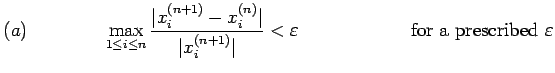
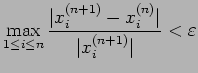$$\max\limits_{1\leq i \leq n}\frac{\vert x_i^{(n+1)}-x_i^{(n)}\vert}{\vert x_i^{(n+1)}\vert} < \varepsilon$$    for some prescribed $$\varepsilon$$

or until $n > M$ for a prescribed integer M.
Convergence
Let us assume that the system to be solved has been expressed in the form

$$X=Bx+c$$ (30)

where B is n x n matrix with elements $b_{ij}$. The Jacobi and Gauss-seidel methods then consist of choosing an arbitrary initial vector $x^{(0)}$ and generating a sequence of approximations $x^{(n)}$ by the iteration

$$x^{(n+1)}=Bx^{(n)}+c,\qquad n=0,1,2,..$$ (31)

on subtracting (30) from (31),we get

$$x^{(n+1)}-x=B(x^n-x)$$

Let $e^{(n)}=x^{(n)}-x$ denote the error in the $n^{th}$ approximation, then we have

$$e^{(n+1)}=Be^{(n)}$$ (32)

$$=B^2e^{(n-1)}=....=B^{(n+1)}e^{(0)}$$

where $e^{(0)}$ is the error in the initial approximation $x^{(0)}$. We must now show that regardless of what the initial error $e^{(0)}$
Theorem: The iteration defined by (31) will converge for any choice of the initial vector $x^{(0)}$ if and only if the eigen values of the matrix B are all less than one in magnitude.
Remark: The rate of convergence depends upon the magnitude of the largest eigen value of B. The smaller this eigen value. The faster the rate of convergence.
This theorem is not, however, very helpful in practice because we will generally not know the eigen values of B.
We shall describe sufficient condition for convergence in the following Theorem, which is more practicable.
Theorem: In the jacobi iteration, let me elements of B satisfy the column sum inequalities

$$\sum\limits_{i=1}^n\vert b_{ij}\vert\leq M < 1\, ,\qquad j=1,2,...,n$$ (33)

Then the Jacobi iteration method will converge for any choice of the initial approximation $x^{(0)}$.
Proof: The error equation (32) can be explicitly written as

$$e_1^{(m+1)}=b_{11}e_1^{(m)}+b_{12}e_2^{(m)}+...+b_{1n}e_n^{(m)}$$

$$e_2^{(m+1)}=b_{21}e_1^{(m)}+b_{22}e_2^{(m)}+...+b_{2n}e_n^{(m)}$$

$$e_n^{(m+1)}=b_{n1}e_1^{(m)}+b_{n2}e_2^{(m)}+...+b_{nn}e_n^{(m)}$$

Taking absolute values and applying the triangle inequality, we have

$$\vert e_1^{(m+1)}\leq \vert b_{11}\vert\,\vert e_1^{(m)}\vert+\vert b_{12}\vert\,\vert e_2^{(m)}\vert+...+\vert b_{1n}\vert\,\vert e_n^{(m)}\vert$$

$$\vert e_2^{(m+1)}\leq \vert b_{21}\vert\,\vert e_1^{(m)}\vert+\vert b_{22}\vert\,\vert e_2^{(m)}\vert+...+\vert b_{2n}\vert\,\vert e_n^{(m)}\vert$$

$$\vert e_n^{(m+1)}\leq \vert b_{n1}\vert\,\vert e_1^{(m)}\vert+\vert b_{n2}\vert\,\vert e_2^{(m)}\vert+...+\vert b_{nn}\vert\,\vert e_n^{(m)}\vert$$

Adding these inequality, we obtain

$$\sum\limits_{i=1}^n\vert e_i^{(m+1)}\vert\leq \vert e_1^{(m)}\ver... ...n\vert b_{i2}\vert+...+\vert e_n^{(m)}\vert\sum\limits_{i=1}^n\vert b_{in}\vert$$

using (32),we get

$$\sum\limits_{i=1}^n\vert e_i^{(m+1)}\vert\leq M \sum\limits_{i=1}^n\vert e_i^{(m)}\vert$$

using this inequalities recursively, we get

$$\sum\limits_{i=1}^n\vert e_i^{(m+1)}\vert\leq M^{m+1} \sum\limits_{i=1}^n\vert e_i^{(0)}\vert$$

Since $M <1$, it follows that

$$\lim\limits_{m\rightarrow \infty} \sum\limits_{i=1}^n\vert e_i^{(m+1)}\vert=0$$

Since this is a finite sum of positive terms, it can vanish only if each term in the sum vanishes separately. We have thus shown that

$$\vert e_i^{(m)}\vert=\vert x_i^{(m)}-x\vert\rightarrow 0$$    as $$m\rightarrow 0 ,\,\,i=1,2,...,n$$

We can also prove the theorem if the elements $b_{ij}$ of B satisfy the row sum inequalities

$$\sum\limits_{j=1}^n\vert b_{ij}\vert\leq M < 1 \qquad i=1,2,...,n$$ (34)

If the condition (34) is satisfied, convergence of Jacobi iteration will take place for any choice of the initial approximation $x^{(0)}$. The conditions (33) and (34) expressed in terms of the elements $a_{ij}$ of A become

$$\sum\limits_{i=1\, i\neq j}^n\vert a_{ij}\vert< \vert a_{jj}\vert\,; \qquad j=1,2,...,n$$ (35)

$$\sum\limits_{j=1\, j\neq i}^n\vert a_{ij}\vert< \vert a_{ii}\vert\,; \qquad i=1,2,...,n$$ (36)

Matrices satisfying condition (36) are said to be strictly diagonally dominant. The conditions given in the theorem are sufficient for convergence but not necessary. These conditions are also sufficient In the convergence for Gauss-serdel method.