
Next: Numerical Differentiation
Up: Main
Previous: The Elimination Method
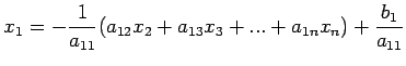
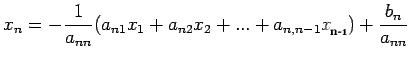
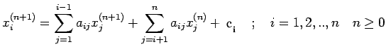
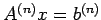
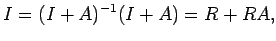
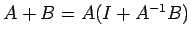
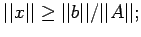
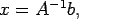
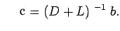
To solve  , we reduce it to an equivalent system
  , in
which U is upper triangular. This system can be easily solved by a
process of backward substitution.
, in
which U is upper triangular. This system can be easily solved by a
process of backward substitution.
Denote the original linear system by
 ,
,
where
![$ A^{(1)}=[a^{(1)}_{ij}],\,\, b^{(1)}=[b_1^{(1)},...b_n^{(1)}]^T
\,\,\, 1\leq i , j\leq n$](img108.png) and n is the order of the system. We
reduce the system to the triangular form by adding
multiples of one equation to another equation, eliminating some
unknown from the second equation. Additional row operations are
used in the modifications given later. We define the algorithm in
the following:
and n is the order of the system. We
reduce the system to the triangular form by adding
multiples of one equation to another equation, eliminating some
unknown from the second equation. Additional row operations are
used in the modifications given later. We define the algorithm in
the following:
Gaussian Elimination Algorithm:
Step 1: Assume

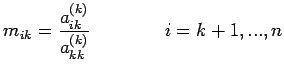
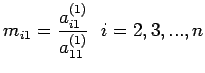
 Define the row multipliers by
These are used in eliminating the  term form equation 2
through n. Define
Also, the first rows of A and b are left undisturbed, and the
first column of
term form equation 2
through n. Define
Also, the first rows of A and b are left undisturbed, and the
first column of  , below the diagonal, is set to zero. The
system
, below the diagonal, is set to zero. The
system
 looks like
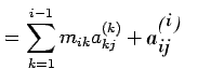
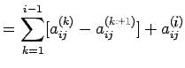
We continue to eliminate unknowns, going onto columns
2, 3, etc., and this is expressed generally as follows.
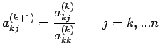
Step

Let
. Assume that
has been constructed with
eliminated at
successive stages and

has the form
Assume
 . Define the multipliers.
 |
(1) |
Use these to remove the unknown's  from equations k+1
through n. Define
from equations k+1
through n. Define
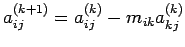 |
(2) |
The earlier rows 1 through k are left undisturbed, and zeros are
introduced into column k below the diagonal element. By continuing
in this manner, after n-1 steps, we obtain
 i.e.
Let
i.e.
Let  and
and  . The system Ux=g is
upper triangular and easy to solve by back substitution; i.e
and
This completes the Gaussian elimination algorithm.
. The system Ux=g is
upper triangular and easy to solve by back substitution; i.e
and
This completes the Gaussian elimination algorithm.
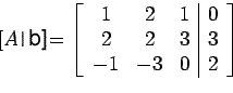
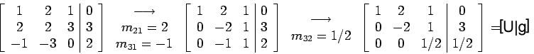
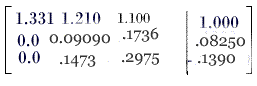
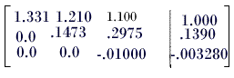
Example: solve the linear system
Represent the linear system by the augmented matrix
and carry out the row operations as given below
Solving Ux=g, We get
Triangular factorization of a matrix
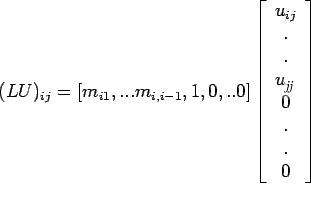
Denote by L the lower triangular matrix given by
Theorem: If L and U are the lower and upper triangular
matrices as defined above, then
Proof: The proof is an algebraic manipulation, making use of (1)
and (2) as given above. We write
For 
For 


This completes the proof.
Corollary: With the matrices A, L and U as in the above theorem.
Proof: Follows by the product rule for determinants
Since L and U are triangular, their determinants are the product
of their diagonal elements. The desired result follows easily,
since det(L)=1.
Example: For the system of the previous example
It is easy to see that A=L U. Also det(A)=det(U)=-1
Pivoting and Scaling in Gaussian Elimination
At each stage of the elimination process given above, we assumed
the appropriate pivot element
 . To remove this
assumption, begin each step of the elimination process by
switching rows to put a non zero element in the pivot position. If
none such exists, then the matrix must be singular, contrary to
assumption.
. To remove this
assumption, begin each step of the elimination process by
switching rows to put a non zero element in the pivot position. If
none such exists, then the matrix must be singular, contrary to
assumption.
It is not enough, however, to just ask that pivot
element be nonzero. Nonzero but very small pivot element will
yield gross errors in further calculation and to guard against
this and propagation of rounding errors, we introduce pivoting
strategies.
Definition: (Partial Pivoting). For
in the Gaussian elimination process at stage k, let
Let i be the smallest row index,

, for which the maximum

is attained. If

then switch rows k and i in A and
b, and proceed with step k of the elimination process. All the
multipliers will now satisfy
This helps in preventing the growth of elements in of
greatly varying size, and thus lessens the possibility for
large
loss of significance errors.
Definition: (Complete Pivoting).
Define
Switch rows of A and b and columns of A to bring to the pivot
position an element giving the maximum
.
However, complete pivoting is more expensive and thus partial
pivoting is more often used
Example: Consider solving the system with and without pivoting:
....................(3)

 ...............(4)
The error in (3) is from seven to sixteen times larger than it is
for (4), depending upon the component of the solution being
considered. The results in (4) have one more significant digit
than those in (3). This illustrates the positive effect that the
use of pivoting can have on the error for Gaussian elimination.
Scaling: It has been observed that if the elements of
the coefficient matrix A vary greatly in size, then it is likely
that large loss of significance errors will be introduced and the
propagation of rounding errors will be worse. To avoid this
problem, we usually scale the matrix A so that the elements vary
less. This is usually done by multiplying the rows and columns by
suitable constants. If we let B denote the result of row and
column scaling in A, then
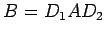
where  and
and  are the diagonal matrices, with entries the scaling constants. To
solve , observe that
are the diagonal matrices, with entries the scaling constants. To
solve , observe that
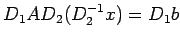
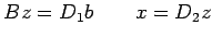
Thus we solve for x by solving
Restricting ourselves to row scaling, we attempt to choose the
coefficients so as to have
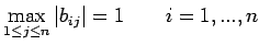
where
![$ B=[b_{ij}]$](img174.png) is the result of scaling A.
is the result of scaling A.
Gauss-Jordan Method
This procedure is much the same as
Gauss elimination including the possible use of pivoting and
scaling. It differs in eliminating the unknown in equation above
the diagonal as well as below it. In step k of the elimination,
choose the pivot element as before. Then define
Eliminate the unknown in equation both above and below
equation k. Define
The procedure will convert the augmented matrix  to
to
 , so that the solution is
  .
.
The Choleski Method
Let A be a symmetric and positive definite matrix of order n. The
matrix is positive definite if
 for all
  . For such a matrix A,
there is a very convenient factorization and can be carried out
without any need for pivoting or scaling. This is called Choleski
factorization and that is we can find a lower triangular real
matrix L such that
. For such a matrix A,
there is a very convenient factorization and can be carried out
without any need for pivoting or scaling. This is called Choleski
factorization and that is we can find a lower triangular real
matrix L such that
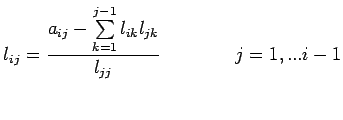
Construction of the matrix L: Let
 with
with
 for
for  . Begin the construction of L by multiplying
the first row of A times the first column of
. Begin the construction of L by multiplying
the first row of A times the first column of  , we get
Because A is positive definite,
, we get
Because A is positive definite,  and
and
 . Next, multiply the second row of L times
the first two columns of to get
Again, we can solve for the unknowns
. Next, multiply the second row of L times
the first two columns of to get
Again, we can solve for the unknowns  and
and  . In
general for
. In
general for
![$\displaystyle l_{ii}=[a_{ii}-\sum\limits_{k=1}^{i-1}l^2_{ik}]^{1/2}$](img197.png) |
(5) |
The square root in (5) of choleski's method can be avoided by
using a slight modification of the factorization. That is to find
a diagonal matrix D and a lower triangular matrix

, with
unity on the diagonal, such that
 |
(6) |
Example: Consider the Hilbert matrix of order 3,
For the choleski decomposition
And for (6), we have
Tridiagonal systems
The matrix
![$ A=[a_{ij}]$](img203.png) is tridiagonal, if
is tridiagonal, if  for
for

Let
Consider  The elements
 and
and  can be computed recursively
as:
These can be solved to give
can be computed recursively
as:
These can be solved to give

A is non-singular)
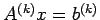
To solve  , let
, let  and
and  . Then
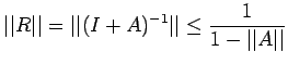
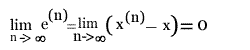
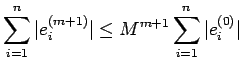
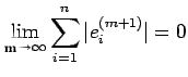
Error Analysis:
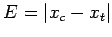
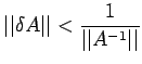
Consider solving the system , where A is a non-singular
matrix of order n. Denote by  and
and  the true and computed
solutions, respectively, of . One possible measure of the
error in the computed solution would be the magnitude of the
residual vector
the true and computed
solutions, respectively, of . One possible measure of the
error in the computed solution would be the magnitude of the
residual vector
If
then
Remark:
But this is not appropriate of error analysis as

can be
quite small even though
is a very erroneous solution. This
can be justified in the following manner: if

has some
large elements, then r may be very small even if
is
substantially different from the true solution. For
or
Therefore, if some elements of
are
large, a small component of r can still mean a large difference
between
and
, or conversely,
may be far from
but r can nevertheless still be small. In other words, an
accurate solution (i.e a small difference between
and
)
will always produce small residuals but small residuals do not
guarantee an accurate solution.
If the system
is such
that
contains some very large elements, then we say the
matrix and, therefore, the system of equations is
ill-conditioned. The following simple example will
illustrate the dangers inherent in solving ill-conditioned system.
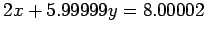
Consider the system
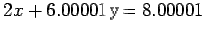 |
(7) |
which has the solution x=1, y=1, and the system
 |
(8) |
which has the solution x=10, y=-2. Here a change of .00002
in

and .00001 in

has caused a gross change in the
solution. The inverse of the matrix of coefficients in (7) has
elements whose order of magnitude is

, which indicates the
ill conditioning of A.
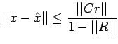
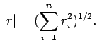
A more reasonable measure of the error is given by
It is this error we shall try to estimate here. Any bound on E
will depend on the magnitude of the round off errors incurred, the
order of the matrix A, and the size of
. One approach to
finding such a bound would be to consider the worst possible case
of round off at each stage of the method and to derive a bound
based on the accumulation of these errors. Since the round off at
one stage is quite complicated function of the round off at
previous stages, such bounds are difficult to calculate. Instead
our approach here will be to estimate the perturbed system of
equations whose true solution is the calculated solution
.
That is, the computed solution
is the true solution of some
system which we write as
 and
and  precisely; our object is to
find bounds on their elements.
precisely; our object is to
find bounds on their elements.
We have
![$\displaystyle \qquad=[(A+\delta A)^{-1}-A^{-1}]b+(I+A^{-1}\delta A)^{-1}A^{-1}\delta
b$](img243.png) |
(9) |
In order to find a bound E, we consider the following two norms of
the matrix A.
i) Euclidean Norm of A is defined as
ii) Spectral Norm of A is defined as
where the notation

denotes an eigen value of

. Both of these norms are defined for any m x n matrix. For
vectors we define the norm in the Euclidean sense as
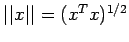
.
The Euclidean norm may also be expressed
as
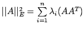 where n is the
order of
where n is the
order of
Thus we have the important result
For our
purpose the spectral norm is much more useful of the two norms. We
shall here after drop the subscript
s on the spectral norm. We
also need to use the spectral radius, which is defined as
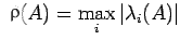
, Thus
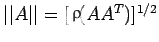
, and when A is symmetric, we have
We need the following theorem to obtain the error bound.
Theorem: Let A be a square matrix and x any vector.
Then
 be the largest eigen value in magnitude of
. For any x
be the largest eigen value in magnitude of
. For any x
Since the eigen value of

are nonpositive
and therefore the numerator is negative semi-definite. Equality
holds when x is an eigen vector of

corresponding to
.
Hence the theorem.
Corollary 1.
 Proof:
 The result follows by letting x be the eigen vector
corresponding to any eigen value of A.
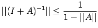
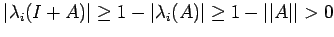
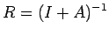
Corollary 2. If

, then I+A is non-singular.
Proof:
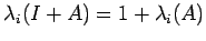
(

the eigen
values of I are 1.) Thus
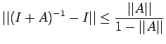
 Corollary 3
. If
,then
where
Taking norm, we have
from which it follows that
The second part also follows easily.
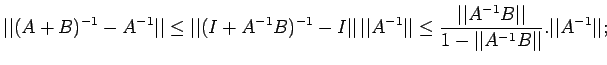
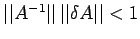
Corollary 4. If A is non-singular and
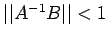 ,
then A+B is nonsingular and
,
then A+B is nonsingular and
where
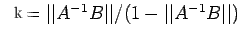 Proof:
 Using corollary 2, the non-singularity of both A+B and

follows since
. We have
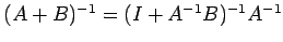
.Thus
![$\displaystyle \leq \frac{\vert\vert A^{-1}\vert\vert}{1-\vert\vert A^{-1}\vert\...
...ert\vert A^{-1}\vert\vert\,\vert\vert b\vert\vert+\vert\vert\delta b\vert\vert]$](img280.png) |
(10) |
where we have assumed that
 . One can
see that bound (10) depends upon bounds on
. One can
see that bound (10) depends upon bounds on
 and
and
 in addition to a bound on
 .
.
A priori Error Estimate
In solving the system
 |
(11) |
by any procedure, round off errors will in general be introduced.
But if the problem is well posed these errors can be kept with in
reasonable bounds. By a problem to be well posed, we mean that
'small' changes in the data lead to 'small' changes in the
solution.
Suppose that the matrix A and b in (11) are perturbed by the quantities
and  . Then if the perturbation in
the solution x of (11) is
. Then if the perturbation in
the solution x of (11) is  , we have
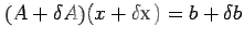 |
(12) |
Now an estimate of the relative change in the solution can be
given in terms of the relative changes in A and b by means of the
following.
Theorem: Let A be non-singular and the perturbation
be so small that
 |
(13) |
Then if x and satisfy (11) and (12), we have
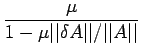
where the condition number  is defined as
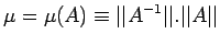 |
(14) |
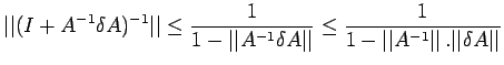
Proof: Since
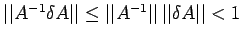 by (13), it follows that by
corollary 2 and 3, the matrix
by (13), it follows that by
corollary 2 and 3, the matrix
 is non singular
and further that
Now multiply (12) by , using (11) and solving for ,
we get
Taking norm and divide by
is non singular
and further that
Now multiply (12) by , using (11) and solving for ,
we get
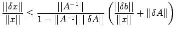
Taking norm and divide by  we get
Now form (11) it is clear that
we get
Now form (11) it is clear that
 this
gives
this
gives
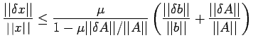
![$\displaystyle \frac{\vert\vert\delta x\vert\vert}{\vert\vert x\vert\vert}\leq \...
...b\vert\vert}+\frac{\vert\vert\delta A\vert\vert}{\vert\vert A\vert\vert}\right]$](img300.png) |
(15) |
which yields the result using the definition (14).
The estimate (15) shows that small relative change in b and A
cause small relative changes in the solution if the factor
is not too large. The condition (13) is equivalent to
 . Thus, it is clear that when
the condition number
. Thus, it is clear that when
the condition number  is not too large, the system (11) is
well conditioned. Note that we can not expect to be small
compared to unity since
A Posteriori Error Estimate
is not too large, the system (11) is
well conditioned. Note that we can not expect to be small
compared to unity since
A Posteriori Error Estimate
Although we do not advocate inverting a matrix to solve linear
system, it is of interest to consider error estimates related to
computed inverses. Let A be the matrix to be inverted and let C be
the computed inverse. The error in the inverse is defined by
 |
(16) |
We also use another measure of error called the residual
matrix:
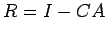 |
(17) |
We have the following result.
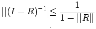
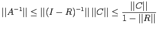
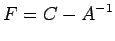
Theorem: If  , then A and C are non-singular, and
Proof: Since , I-R is non-singular(by an earlier
theorem) and
Now
, then A and C are non-singular, and
Proof: Since , I-R is non-singular(by an earlier
theorem) and
Now 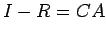
and thus both det(C) and det(A) are non zero. This proves that
both A and C are non singular. Now
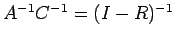 or
and
Also
and
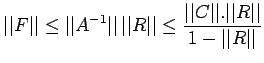
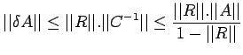
Corollary:
or
and
Also
and
Corollary:
If is of interest to note that with C an approximate inverse of A,
we can find the perturbation so that C is the exact
inverse of
 . That is,
or
and
Finally, we observe that the computed inverse can also be used to
estimate the error in solving a linear system. This is given in
the following.
. That is,
or
and
Finally, we observe that the computed inverse can also be used to
estimate the error in solving a linear system. This is given in
the following.
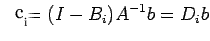
Theorem: Let A, C and R be as given in the previous
theorem. Let  be an approximate solution to Ax=b and
define
be an approximate solution to Ax=b and
define
 . Then
Proof.
or
and
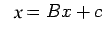
Iterative methods
. Then
Proof.
or
and
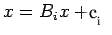
Iterative methods
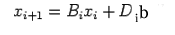
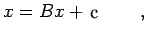
We restrict to linear iteration which has the form
 |
(18) |
where the matrix  and vector
  are independent of
  in
a stationary iteration.
in
a stationary iteration.
To motivate considering iterations of the type (18), to solve
|
(19) |
let us write (19) in the form
or
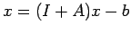 |
(20) |
Equation (20) suggests the iteration
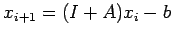 |
(21) |
Equation(18) is then just a generalization of (21). We require
that the true solution x of (19) be a fixed point of (18). We must
then have
for all

 we have
or
we have
or
 |
(22) |
We assume that and  are independent of b. Therefore, we
must have
or
are independent of b. Therefore, we
must have
or
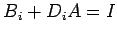 |
(23) |
This is called the
condition of consistency for and . In view of (22), we
can write (18) in the form
 |
(24) |
To consider
the convergence of (24), we define
 . Thus
, (using (23) )
If  is the initial approximation to the solution of (19),
then
where
is the initial approximation to the solution of (19),
then
where
 |
(25) |
Therefore, a necessary and sufficient condition for the
convergence of the sequence  to x for arbitrary is
that
to x for arbitrary is
that
for all

While a sufficient condition for convergence is that
We also have
 Therefore,
 is also a
sufficient condition for the convergence of the iteration (18). For
stationary iterative process still another sufficient condition for
convergence is
is also a
sufficient condition for the convergence of the iteration (18). For
stationary iterative process still another sufficient condition for
convergence is
 |
(26) |
When an iteration is stationary, then
 and from (25), we have
The eigen values of
 and the
 powers of the eigen values of B.
Therefore, the condition (26) is equivalent to requiring that all
eigen values of B lie with in the unit circle. In fact, this is a
necessary and sufficient condition for the convergence of
stationary iteration.
powers of the eigen values of B.
Therefore, the condition (26) is equivalent to requiring that all
eigen values of B lie with in the unit circle. In fact, this is a
necessary and sufficient condition for the convergence of
stationary iteration.
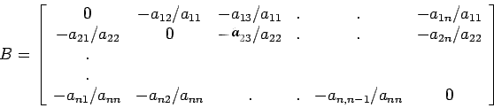
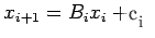
The Jacobi Iteration
We write the matrix A in the form
Where D is a
diagonal matrix with
 and L and U are, respectively,
lower and upper triangular matrices with zeros on the diagonal.
Then the system
can be written as
and L and U are, respectively,
lower and upper triangular matrices with zeros on the diagonal.
Then the system
can be written as
 |
(27) |
We now define the iteration
 |
(28) |
where  is an initial approximation. This is known as
Jacobi iteration or the method of simultaneous displacements.
is an initial approximation. This is known as
Jacobi iteration or the method of simultaneous displacements.
If
 , we can write (27) in the component form as
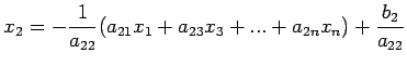 |
(29) |
.
.
.
If we let
then (29) can be written as
where
Algorithm: Let the system be expressed in the
form
where B is an n x n matrix as given above and c is
a given column vector. To find an approximate solution.
1. Choose an arbitrary initial approximation vector . If
no better choice is available, choose

for

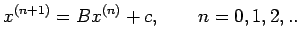
2. Generate successive approximation
 by the iteration
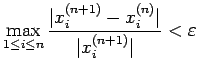
3. Continue until either of the following convergence criteria is
satisfied.
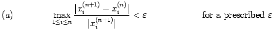
or
 for a prescribed
integer M
for a prescribed
integer M 
Example: A simple example illustrating Jacobi
iteration is the following:
The exact solution is
 . To
solve it by Jacobi iteration, we write it in the form
Choosing
. To
solve it by Jacobi iteration, we write it in the form
Choosing
 we obtain successive approximations and, for example,
we get
which is a good approximation for the exact solution.
we obtain successive approximations and, for example,
we get
which is a good approximation for the exact solution.
Gauss-Seidel iteration (Method of successive
displacement):
We split the system as
and write
or
where
and
where  is an initial approximation. The algorithm for Gauss-seidel
method is given below:
is an initial approximation. The algorithm for Gauss-seidel
method is given below:
Algorithm:
1. Choose an arbitrary initial approximation vector
2. Generate successive approximations
by the iteration
for some prescribed

 for a prescribed integer M.
Convergence
Let us assume that the system to be solved has been expressed in
the form
 |
(30) |
where B is n x n matrix with elements  . The Jacobi and
Gauss-seidel methods then consist of choosing an arbitrary initial
vector and generating a sequence of approximations
by the iteration
. The Jacobi and
Gauss-seidel methods then consist of choosing an arbitrary initial
vector and generating a sequence of approximations
by the iteration
 |
(31) |
on subtracting (30) from (31),we get
Let
 denote the error in the
  approximation, then we have
 |
(32) |
 |
(33) |
Then the Jacobi iteration method will converge for any choice of
the initial approximation .
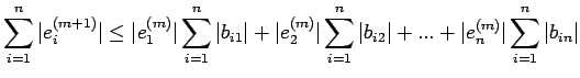
Proof: The error equation (32) can be explicitly
written as
Taking absolute values and applying the triangle inequality, we
have
.
.
.
.
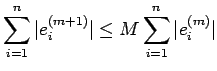
Adding these inequalities, we obtain
using (32),we get
using this inequality recursively, we get
Since  , it follows that
Since this is a finite sum of positive terms, it can vanish only
if each term in the sum vanishes separately. We have thus shown
that
, it follows that
Since this is a finite sum of positive terms, it can vanish only
if each term in the sum vanishes separately. We have thus shown
that
as
We can also prove the theorem if the elements of B
satisfy the row sum inequalities
 |
(34) |
If the condition (34) is satisfied, convergence of Jacobi
iteration will take place for any choice of the initial
approximation . The conditions (33) and (34) expressed in
terms of the elements  of A become
 |
(35) |
 |
(36) |
Matrices satisfying condition (36) are said to be strictly
diagonally dominant. The conditions given in the theorem are
sufficient for convergence but not necessary. These conditions are
also sufficient in the convergence for Gauss-seidel method.
Exercises
Next: Numerical Differentiation
Up: Main
Previous: The Elimination Method
![\begin{displaymath}\left[%
\begin{array}{ccccc}
a_{11}^{(1)} & a_{12}^{(1)} &...
...} \\
. \\
. \\
b_{n}^{(2)} \\
\end{array}%
\right] \end{displaymath}](img115.png)
![\begin{displaymath}A^{(k)}=\left[%
\begin{array}{cccccccc}
a_{11}^{(1)} & a_{...
..._{nk}^{(k)} & . & . & a_{nn}^{(k)} \\
\end{array}%
\right]
\end{displaymath}](img120.png)
![\begin{displaymath}\left[%
\begin{array}{ccccc}
a_{11}^{(1)} & . & . & . & a_...
... . \\
. \\
. \\
b_{n}^{(n)} \\
\end{array}%
\right]\end{displaymath}](img127.png)

![$\displaystyle x_k=\frac{1}{u_{kk}}[g_k- \sum\limits_{j=k+1}^n u_{kj}x_j]\,\,\,\ , \, k=n-1,n-2, ...1$](img131.png)
![\begin{displaymath}L=\left[%
\begin{array}{cccccc}
1 & 0 & 0 & . & . & 0 \\
...
...\
m_{n1} & m_{n2} & . & . & . & 1 \\
\end{array}%
\right]\end{displaymath}](img138.png)
![\begin{displaymath}L=
\left[%
\begin{array}{ccc}
1 & 0 & 0 \\
2 & 1 & 0 \...
...\\
0 & -2 & 1 \\
0 & 0 & 1/2 \\
\end{array}%
\right]
\end{displaymath}](img149.png)
![\begin{displaymath}\left[%
\begin{array}{ccc\vert c}
.7290 & .8100 & .9000 & ...
... \\
1.331 & 1.210 & 1.100 & 1.000 \\
\end{array}%
\right]\end{displaymath}](img160.png)
![\begin{displaymath}\left[%
\begin{array}{ccc\vert c}
.7290 & .8100 & .9000 & ...
...\\
0.0 & -.2690 & -.5430 & -.2540 \\
\end{array}%
\right]\end{displaymath}](img162.png)
![\begin{displaymath}\left[%
\begin{array}{ccc\vert c}
.7290 & .8100 & .9000 & ...
...4 \\
0.0 & 0.0 & .02640 & .008700 \\
\end{array}%
\right]\end{displaymath}](img164.png)

![\begin{displaymath}A=\left[%
\begin{array}{ccc}
1 & 1/2 & 1/3 \\
1/2 & 1/3 & 1/4 \\
1/3 & 1/4 & 1/5 \\
\end{array}%
\right]\end{displaymath}](img200.png)
![\begin{displaymath}
L=\left[%
\begin{array}{ccc}
1 & 0 & 0 \\
1/2 & 1/2\s...
...
1/3 & 1/2\sqrt{3} & 1/6\sqrt{5} \\
\end{array}%
\right] \end{displaymath}](img201.png)
![\begin{displaymath}\hat{L}=\left[%
\begin{array}{ccc}
1 & 0 & 0 \\
1/2 & 1...
...
0 & 1/12 & 0 \\
0 & 0 & 1/180 \\
\end{array}%
\right]
\end{displaymath}](img202.png)
![\begin{displaymath}A=\left[%
\begin{array}{ccccccc}
a_1 & c_1 & 0 & 0 & . & ....
...b_n & a_n \\
\end{array}%
\right],\mbox{ with } det(A)\neq 0\end{displaymath}](img205.png)
![\begin{displaymath}=\left[%
\begin{array}{cccccc}
\alpha_1 & 0 & . & . & . & ...
... & 1 & r_{n-1} \\
& & & & 0 & 1 \\
\end{array}%
\right]
\end{displaymath}](img207.png)