Next: About this document ...
Up: 2.3 Newton Interpolation Polynomial
Previous: 2.3.1 Gregory-Newton Forward Difference
If the data size is big then the divided difference table will be
too long. Suppose the desired intermediate value
 at which one needs to estimate the function
 falls towards the end or say in the
second half of the data set then it may be better to start the
estimation process from the last data set point. For thus we need
to use backward-differences and backward difference table.
falls towards the end or say in the
second half of the data set then it may be better to start the
estimation process from the last data set point. For thus we need
to use backward-differences and backward difference table.
Let
us first define backward differences and generate backward
difference table, say for the data set
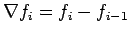
First order backward difference
 is defined as:
 |
(11.1) |
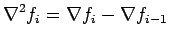
Second order backward difference
 is defined as:
 |
(11.2) |
In general, the  order backward difference is defined as
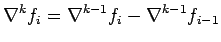 |
(11.3) |
In this case the reference point is  and therefore we can
derive the Newton-Gregory backward difference interpolation
polynomial as:
and therefore we can
derive the Newton-Gregory backward difference interpolation
polynomial as:
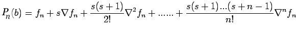 |
(12) |
Where

For constructing
 as given in
  it will be easier if we first
generate backward-difference table. The backward difference table
for the data
it will be easier if we first
generate backward-difference table. The backward difference table
for the data
 is given below:
Newton Backward Difference Table:
Now let us
apply Newton Backward difference approach to the second example
solved earlier following the Newton forward difference approach
i.e.
Example:
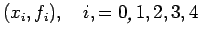
Given the following data estimate  using Newton-Gregory backward difference interpolation polynomial:
| i |
0 |
1 |
2 |
3 |
4 |
5 |
 |
0 |
1 |
2 |
3 |
4 |
5 |
 |
1 |
2 |
4 |
8 |
16 |
32 |
Solution:
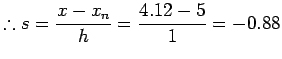
Here
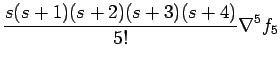
 Newton Backward Difference polynomial
  is
given by
is
given by
Let us first generate backward difference table:
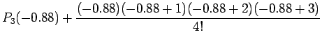
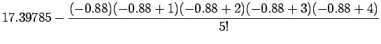
=17.39135 (13.5)
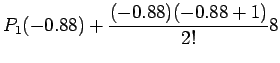
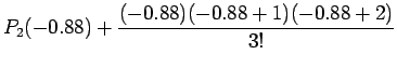
Now for comparison with the earlier solution i.e. the one obtained
by forward Newton Divided Difference approach we may look at the
above solution in stages similar to that provided earlier i.e.
Now one may note from (13.2) and (10a.2) that it is definitely
advantageous of use backward difference approach here, as in
exactly the same number of steps we are relatively more close to
the approximate solution.
Next: About this document ...
Up: 2.3 Newton Interpolation Polynomial
Previous: 2.3.1 Gregory-Newton Forward Difference
root
2006-02-14