Lagrange Interpolation:

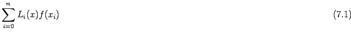
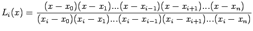
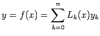
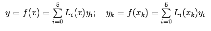
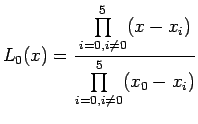
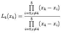
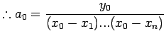
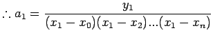
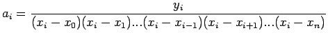
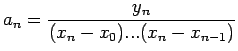
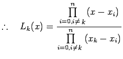
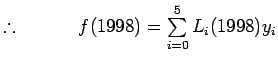
Let us suppose that the given data points $(x_{i},y_{i}),$ $i=0,1,2...n$ is coming from a function $f(x)$. Let us assume that this function $y=f(x)$ takes the values $y_{0},y_{1}.......y_{n}$ at $x_{0},x_{1},.......x_{n}.$ Since there are $(n+1)$ data points $(x_{i},y_{i}),$ we can represent the function $f(x)$ by a polynomial of degree $n.$

$$\therefore f(x)=C_{n}x^{n}+C_{n-1}x^{n-1}+...+C_{1}x+C_{0}$$ (1)

As we have assumed that $f(x_{i})=y_{i}, i=0,1,2.......n$ i.e. the function $f(x)$ passes through $(x_{i}, y_{i}).\quad (1)$ can be rewritten as:

$$y = f(x)= a_{0}(x-x_{1})(x-x_{2})...(x-x_{n})+ a_{1}(x-x_{0})(x-x_{2})...(x-x_{n})+$$

$$a_{2}(x-x_{0})(x-x_{1})(x-x_{3})...(x-x_{n})+.......+ a_{n}(x-x_{0})...(x-x_{n-1})$$ (2)

$$But, y_{i}=f(x_{i})\quad i=0,1,.....n\qquad\qquad\qquad\qquad\qquad\qquad\qquad\qquad\qquad\qquad\qquad\qquad\qquad\qquad\qquad\quad$$ (3)

Using (3) for i=0, in (2) we get

$$y_{0}=f(x_{0})=a_{0}(x_{0}-x_{1})...(x_{0}-x_{n})$$

$$\therefore a_{0}=\frac{y_{0}}{(x_{0}-x_{1})...(x_{0}-x_{n})}$$ (4.1)

For $i=1,$ we get

$$y_{1}=f(x_{1})=a_{1}(x_{1}-x_{o})(x_{1}-x_{2})...(x_{1}-x_{n})$$

$$\therefore a_{1}=\frac{y_{1}}{(x_{1}-x_{0})(x_{1}-x_{2})...(x_{1}-x_{n})}$$ (4.2)

Similarly for $i=2.......n-1,$ we get

$$a_{i}=\frac{y_{i}}{(x_{i}-x_{0})(x_{i}-x_{1})...(x_{i}-x_{i-1})(x_{i}-x_{i+1})...(x_{i}-x_{n})}$$

and for $i=n,$ we get

$$a_{n}=\frac{y_{n}}{(x_{n}-x_{0})...(x_{n}-x_{n-1})}$$ (4.3)

Using (4.1)-(4.3) in (2) we get

$$y=f(x)=\frac{(x-x_{1})(x-x_{2})...(x-x_{n})}{(x_{0}-x_{1})(x_{0}-... ...})...(x-x_{n})}{(x_{1}-x_{0})(x_{1}-x_{2})...(x_{1}-x_{n})}y_{1}+...... ......+$$

$$\frac{(x-x_{0})(x-x_{2})...(x-x_{i-1})(x-x_{i+1})...(x-x_{n})}{(x... ...{0})(x-x_{1})...(x-x_{n-1})}{(x_{n}-x_{0})(x_{n}-x_{1})...(x_{n}-x_{n-1})}y_{n}$$ (5)

(5) can be rewritten in a compact form as:

$$y=f(x) = L_{0}(x)y_{0}+L_{1}(x)y_{1}+...........+L_{n}(x)y_{n}$$

$$= \sum\limits_{i=0}^{n}L_{i}(x)y_{i}$$

$$= \sum\limits_{i=0}^{n}L_{i}(x)f(x_{i})\quad \qquad\qquad\qquad\qquad\qquad\qquad\qquad\qquad\qquad\qquad\qquad\qquad\qquad\qquad(7.1)$$

where

$$L_{i}(x)=\frac{(x-x_{0})(x-x_{1})...(x-x_{i-1})(x-x_{i+1})...(x-x... ...)}{(x_{i}-x_{0})(x_{i}-x_{1})...(x_{i}-x_{i-1})(x_{i}-x_{i+1})...(x_{i}-x_{n})}$$ (7.2)

It can be easily noted that

$$L_{i}(x_{j})=\left\{\begin{aligned}1 \,\, if \,\,i=j\\ 0 \,\, if \,\, i \neq j \end{aligned}\right.$$

Let us introduce the product notation as

$$\prod(x)=\prod\limits_{i=0}^{n}(x-x_{i})=(x-x_{0})(x-x_{1})....(x-x_{n})$$ (8.1)

$$\therefore\quad L_{k}(x)=\frac{\prod\limits_{i=0,i\neq K}^n(x-x_{i})}{\prod\limits_{i=0,i\neq K}^n(x_{k}-x_{i})}$$ (8.2)

Therefore, Lagrange interpolation polynomial of degree n can be written as

$$y=f(x)=\sum\limits_{k=0}^{n}L_{k}(x)y_{k}$$ (9)

Example 1:
Given the following data table, construct the Lagrange interpolation polynomial $f(x)$, to fit the data and find $f(1.25).$

i	0	1	2	3
$x_{i}$	0	1	2	3
$y_{i}=f(x_{i})$	1	2.25	3.75	4.25

Solution:

Here $n=3$.

$\therefore$ Lagrange interpolation polynomial is given by

$$y=f(x) = \sum\limits_{i=0}^{3}L_{i}(x)y_{i}$$

$$L_{0}(x) = \frac{\prod\limits_{i=0,i\neq0}^{3}(x-x_{i})}{\prod\limits_{i=0,i\neq0}^{3}(x_{0}-x_{i})}$$

$$= \frac{(x-x_{1})(x-x_{2})(x-x_{3})}{(x_{0}-x_{1})(x_{0}-x_{2})(x_{0}-x_{3})}$$

$$= \frac{(x-1)(x-2)(x-3)}{(0-1)(0-2)(0-3)}$$

$$= \frac{x^{3}-6x^{2}+11x-6}{-6}$$

$$L_{1}(x) = \frac{\prod\limits_{i=0,i\neq1}^{3}(x-x_{i})}{\prod\limits_{i=0,i\neq1}^{3}(x_{1}-x_{i})}$$

$$= \frac{(x-x_{0})(x-x_{2})(x-x_{3})}{(x_{1}-x_{0})(x_{1}-x_{2})(x_{1}-x_{3})}$$

$$= \frac{(x-0)(x-2)(x-3)}{(1-0)(1-2)(1-3)}$$

$$= \frac{x^{3}-5x^{2}+6x}{2}$$

$$L_{2}(x) = \frac{\prod\limits_{i=0,i\neq2}^{3}(x-x_{i})}{\prod\limits_{i=0,i\neq2}^{3}(x_{2}-x_{i})}$$

$$= \frac{(x-x_{0})(x-x_{1})(x-x_{3})}{(x_{2}-x_{0})(x_{2}-x_{1})(x_{2}-x_{3})}$$

$$= \frac{(x-0)(x-1)(x-3)}{(2-0)(2-1)(2-3)}$$

$$= \frac{x^{3}-4x^{2}+3x}{-2}$$

$$L_{3}(x) = \frac{\prod\limits_{i=0,i\neq3}^{3}(x-x_{i})}{\prod\limits_{i=0,i\neq3}^{3}(x_{3}-x_{i})}$$

$$= \frac{(x-x_{0})(x-x_{1})(x-x_{2})}{(x_{3}-x_{0})(x_{3}-x_{1})x_{3}-x_{2})}$$

$$= \frac{(x-0)(x-1)(x-2)}{(3-0)(3-1)(3-2)}$$

$$= \frac{x^{3}-3x^{2}+2x}{6}$$

$$\therefore \quad f(1.25) = \sum\limits_{i=0}^{3}L_{i}(1.25)y_{i}$$

$$= L_{0}(1.25)y_{0}+L_{1}(1.25)y_{1}+L_{2}(1.25)y_{2}+L_{3}(1.25)y_{3}$$

$$= (-0.546875).1+(0.8203125)2.25+(0.2734375)3.75+(-0.0390625)4.25$$

$$= 2.650390625$$

Example 2:
Given the following data table, construct the Lagrange interpolation polynomial f(x), to fit the data and find $f(1998).$

i	0	1	2	3	4	5
$x_{i}$	1980	1985	1990	1995	2000	2005
$y_{i}=f(x_{i})$	440	510	525	571	500	600

Solution:
Here $n=6,\qquad x_{k}=1998$

$\therefore$ Lagrange interpolation polynomial is given by
$\because y=f(x)=\sum\limits_{i=0}^{5}L_{i}(x)y_{i};\quad y_{k}=f(x_{k})=\sum\limits_{i=0}^{5}L_{i}(x_{k})y_{i}$

$$L_{0}(x)=\frac{\prod\limits_{i=0,i\neq0}^{5}(x-x_{i})}{\prod\limits_{i=0,i\neq0}^{5}(x_{0}-x_{i})} = \frac{(x-x_{1})(x-x_{2})(x-x_{3})(x-x_{4})(x-x_{5})}{(x_{0}-x_{1})(x_{0}-x_{2})(x_{0}-x_{3})(x_{0}-x_{4})(x_{0}-x_{5})}$$

$$= \frac{(x-1985)(x-1990)(x-1995)(x-2000)(x-2005)}{(1980-1985)(1980-1990)(1980-1995)(1980-2000)(1980-2005)}$$

$$L_{0}(x_{k})={L_{0}(1998)} = \frac{(1998-1985)(1998-1990)(1998-1995)(1998-2000)(1998-2005)}{(-5)(-10)(-15)(-20)(-25)}$$

$$= \frac{13.8.3.(-2).(-7)}{-(375000)}$$

$$= -\frac{4368}{375000}=-0.011648$$

$$L_{1}(x_{k})=\frac{\prod\limits_{i=0,i\neq1}^{5}(x_{k}-x_{i})}{\prod\limits_{i=0,i\neq1}^{5}(x_{1}-x_{i})} = \frac{(x_{k}-x_{0})(x_{k}-x_{2})(x_{k}-x_{3})(x_{k}-x_{4})(x_{k}-x_{5})}{(x_{1}-x_{0})(x_{1}-x_{2})(x_{1}-x_{3})(x_{1}-x_{4})(x_{1}-x_{5})}$$

$$= \frac{(1998-1980)(1998-1990)(1998-1995)(1998-2000)(1998-2005)}{(1985-1980)(1985-1990)(1985-1995)(1985-2000)(1985-2005)}$$

$$= \frac{18.8.3.(-2).(-7)}{5(-5)(-10)(-15)(-20)}=0.08064$$

$$L_{2}(x_{k})=\frac{\prod\limits_{i=0,i\neq2}^{5}(x_{k}-x_{i})}{\prod\limits_{i=0,i\neq2}^{5}(x_{2}-x_{i})} = \frac{(1998-1980)(1998-1985)(1998-1995)(1998-2000)(1998-2005)}{(1990-1980)(1990-1985)(1990-1995)(1990-2000)(1990-2005)}$$

$$= \frac{18.13. 3 .(-2)(-7)}{10.5.(-5)(-10).(-15)}$$

$$= -0.26208$$

$$L_{3}(x_{k})=\frac{\prod\limits_{i=0,i\neq3}^{5}(x_{k}-x_{i})}{\prod\limits_{i=0,i\neq3}^{5}(x_{3}-x_{i})} = \frac{(1998-1980)(1998-1985)(1998-1990)(1998-2000)(1998-2005)}{(1995-1980)(1995-1985)(1995-1990)(1995-2000)(1995-2005)}$$

$$= \frac{18.13.8.(-2)(-7)}{15.10.5(-5)(-10)}$$

$$= 0.69888$$

$$L_{4}(x_{k})=\frac{\prod\limits_{i=0,i\neq4}^{5}(x_{k}-x_{i})}{\prod\limits_{i=0,i\neq4}^{5}(x_{4}-x_{i})} = \frac{(1998-1980)(1998-1985)(1998-1990)(1998-1995)(1998-2005)}{(2000-1980)(2000-1985)(2000-1990)(2000-1995)(2000-2005)}$$

$$= \frac{18.13.8.3.(-7)}{20.15.10.5(-5)}$$

$$= 0.52416$$

$$L_{5}(x_{k})=\frac{\prod\limits_{i=0,i\neq5}^{5}(x_{k}-x_{i})}{\prod\limits_{i=0,i\neq5}^{5}(x_{5}-x_{i})} = \frac{(1998-1980(1998-1985)(1998-1990)(1998-1995)(1998-2000)}{(2005-1980)(2005-1985)(2005-1990)(2005-1995)(2005-2000)}$$

$$= \frac{18.13.8.3.(-2)}{25.20.15.10.5}=-0.029952$$

$\therefore \hspace{0.5in} f(1998)=\sum\limits_{i=0}^{5}L_{i}(1998)y_{i}$
$\hspace{1in}=-0.011648 \times 440 + 0.08064 \times 510 + -0.26208 \times 525 + 0.69888 \times 571 + 0.52416 \times 500 + 0.029952 \times 600$
$=541.578560$

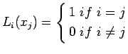
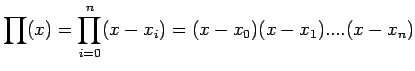
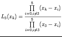
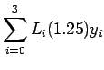
Note: Given a set of data points $(x_{i},y_{i})\qquad i=1,...n$. Suppose we are interested in evaluating $f(x)$ at some intermediate point $x$ to a desired level of accuracy. Directly using the entire data set of size n may not only be computationally economical but may also turn out to be redundant. Naturally one would like to use a interpolating polynomial of apt degree. Since this is not known a priori, one may start with $p_{o}(x)$ and if it was enough then move onto $p_{1}(x)$ and so on i.e. slowly increase the no. of the interpolating points (or) data points $x_{0},x_{1}..x_{k}$ so that $p_{k-1}(x)$ will be close to $f(x)$. In this context the biggest disadvantage with Lagrange Interpolation is that we cannot use the work that has already been done i.e. we cannot make use of $p_{k-1}(x)$ while evaluating $p_{k}(x)$. With the addition each new data point, calculations have to be repeated. Newton Interpolation polynomial overcomes this drawback.