Next: Definitions and Examples Up: Laplace Transform Previous: Laplace Transform Contents
In many problems, a function
![]() is transformed to
another function
is transformed to
another function ![]() through a relation of the type:
through a relation of the type:
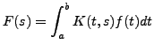
where
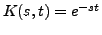 ). As we will see in the following, application of Laplace
transform reduces a linear differential equation with constant coefficients
to an algebraic equation, which can be solved by algebraic methods.
Thus, it provides a
powerful tool to solve differential equations.
). As we will see in the following, application of Laplace
transform reduces a linear differential equation with constant coefficients
to an algebraic equation, which can be solved by algebraic methods.
Thus, it provides a
powerful tool to solve differential equations.
It is important to note here that there is some sort of analogy with what
we had learnt during the study of logarithms in school. That is, to multiply
two numbers, we first calculate their logarithms, add them and then use
the table of antilogarithm to get back the original product. In a similar
way, we first transform the problem that was posed as a function of ![]() to a problem in
to a problem in ![]() , make some calculations and then use the table of
inverse Laplace transform to get the solution of the actual problem.
, make some calculations and then use the table of
inverse Laplace transform to get the solution of the actual problem.
In this chapter, we shall see same properties of Laplace transform and its applications in solving differential equations.
A K Lal 2007-09-12