Numerical Methods

All said and done, the Picard's Successive approximations is not suitable for computations on computers. In the absence of methods for closed form solution (in the explicit form), we wish to explore ``how computers can be used to find approximate solutions of IVP" of the form

$$y^\prime = f(x,y), \hspace{1in} y(x_0) = y_0.$$ (7.7.1)

In this section, we study a simple method to find the ``numerical solutions" of (7.7.1). The study of differential equations has two important aspects (among other features) namely, the qualitative theory, the latter is called "Numerical methods" for solving (7.7.1). What is presented here is at a very rudimentary level nevertheless it gives a flavour of the numerical method.

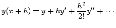
To proceed further, we assume that $f$ is a ``good function" (there by meaning ``sufficiently differentiable"). In such case, we have

$$y(x+h) = y + h y^\prime + \frac{h^2}{2!} y^{\prime\prime} + \cdots$$

which suggests a ``crude" approximation $y(x+h) \simeq y + h f(x, y)$ (if $h$ is small enough), the symbol $\simeq$ means ``approximately equal to". With this in mind, let us think of finding $y,$ where $y$ is the solution of (7.7.1) with $x > x_0.$ Let $h = \displaystyle\frac{x - x_0}{n}$ and define

$$x_i = x_0 + i h, \;\; i=0,1,2,\ldots, n.$$

That is, we have divided the interval $[x_0, x]$ into $n$ equal intervals with end points $x_0, x_1, \ldots, x = x_n.$

Figure 7.1: Partitioning the interval

Our aim is to calculate $y: \;\;$ At the first step, we have $y(x+h) \simeq y_0 + h f\bigl(x_0, y_0\bigr).$ Define $y_1 = y_0 + h f(x_0, y_0).$ Error at first step is

$$\vert y(x_0+h) - y_1 \vert = E_1.$$

Similarly, we define $y_2 = y_1 + h f(x_1, y_1)$ and we approximate $y(x_0 + 2 h) = y(x_2) \simeq y_1 + h f(x_1, y_1) = y_2$ and so on. In general, by letting $y_k = y_{k-1} + h f(x_{k-1}, y_{k-1}),$ we define (inductively)

$$y(x_0 + (k+1) h) = y_{k+1} \simeq y_k + h f(x_k, y_k), \hspace{1in} k = 0, 1, 2, \ldots, n-1.$$

This method of calculation of $y_1, y_2, \ldots, y_n$ is called the Euler's method. The approximate solution of (7.7.1) is obtained by ``linear elements" joining $(x_0, y_0), (x_1, y_1), \ldots, (x_n, y_n).$

Figure 7.2: Approximate Solution