Next: Algorithm for Predictor-Corrector Method Up: Numerical Methods Previous: Runge-Kutta Method of Order Contents
In Sections ![]() and
and ![]() , during the course of the discussion on the Euler's algorithm, the value of
, during the course of the discussion on the Euler's algorithm, the value of
 has been approximated to
![]() . On the other hand, we could
have also considered its approximate value by
. On the other hand, we could
have also considered its approximate value by
 .
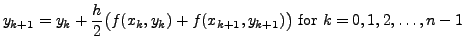
We could have thought of it to solve the IVP (numerically) by defining the approximations
.
We could have thought of it to solve the IVP (numerically) by defining the approximations
![[*]](crossref.png) ) for
) could be too tough and so we resort to (numerical) approximate value for
) for
) could be too tough and so we resort to (numerical) approximate value for

is ``small" (small have means that the absolute value of the ratio is lesser than an assigned (previously) small number). we repeat the process with
) allows us to recursively define
for
 .
The iterated values
.
The iterated values
 .
.
Some more terminologies:
Normally, an explicit method like the
Euler's method or the R-K methods are known as open type methods or algorithms. They are
readily available for computation and the starters are known. On the other hand, implicit method as described
by () is called closed type. Many a times, it may happen that the starters
for the (approximate solution) for closed type method is obtained from the open type one. The starter
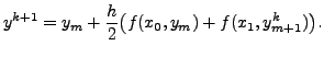
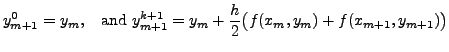
![]() for () is also familiarly known as a Predictor whereas the value
for () is also familiarly known as a Predictor whereas the value ![]() (so computed) is called a corrector. In short, we predict the value
(so computed) is called a corrector. In short, we predict the value ![]() and correct it
(by iteration) to obtain
and correct it
(by iteration) to obtain ![]() . For this reason such methods are called PREDICTOR-CORRECTOR MEHTODS,
(in short PC methods). Again, we repeat that PC methods need some condition to step the inner
iterations, usually they are:
. For this reason such methods are called PREDICTOR-CORRECTOR MEHTODS,
(in short PC methods). Again, we repeat that PC methods need some condition to step the inner
iterations, usually they are:
is concerned, it simply says we do not wish to iterate
beyond says that keep iterating till the relative error
is small, no matter how many iterations are needed. The number and to stop the inner iterations,
which even leads to early termination.
With these preliminaries, we state the Predictor-Corrector algorithm.