Next: Numerical Differentiation and Integration Up: Lagrange's Interpolation Formula Previous: Lagrange's Interpolation formula Contents
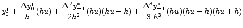
![$\displaystyle \delta[x_0^*,x_1^*] = \frac{\Delta y_0^*}{h}, \hspace{.25in}
\del...
...x_1^*,x_{-1}^*] = \delta[x_{-1}^*,x_0^*,x_1^*]=\frac{\Delta^2
y_{-1}^* }{2h^2},$](img5313.png) |
|||
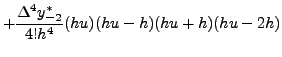
![$\displaystyle \delta[x_0^*,x_1^*,x_{-1}^*,x_2^*] = \delta[x_{-1}^*,x_0^*,x_1^*,x_2^*
]=\frac{\Delta^3 y_{-1}^* }{3!h^3},$](img5314.png) |
|||
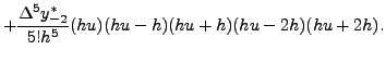
![$\displaystyle \delta[x_0^*,x_1^*,x_{-1}^*,x_2^*,x_{-2}^*] = \delta[x_{-2}^*,
x_{-1}^*,x_0^*,x_1^*,x_2^* ]=\frac{\Delta^4 y_{-2}^* }{4!h^4},$](img5315.png) |
|||
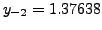
![$\displaystyle \delta[x_0^*,x_1^*,x_{-1}^*,x_2^*,x_{-2}^*,x_3^*] =
\delta[x_{-2}^*,x_{-1}^*,x_0^*,x_1^*,x_2^*,x_3^* ]=\frac{\Delta^5
y_{-2}^* }{5!h^5},$](img5316.png) |
 |
|||
 |
|||
 |
|
|
0.20 | 0.21 | 0.22 | 0.23 | 0.24 |
| |
1.37638 | 1.28919 | 1.20879 | 1.13427 | 1.06489 |
Here the point ![]() lies near the central tabular point
lies near the central tabular point
![]() Thus , we define
Thus , we define
 to get the difference table in diagonal form as:

|
|
|||||
|
|
||||||

|
|
|
||||
|
|
|
|||||

|
|
|
|
|||
|
|
|
|||||

|

|
|
||||
|
|
||||||

|
|
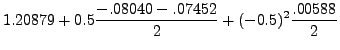
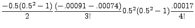
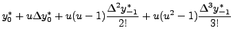
Using the Sterling's formula with
 we get
 ![]() as follows:
as follows:
 |
|||
 |
|||
Note that tabulated value of
![]() at
at ![]() is
1.1708496.
is
1.1708496.
|
|
0.00 | 0.02 | 0.04 | 0.06 | 0.08 |
| |
0.00000 | 0.02256 | 0.04511 | 0.06762 | 0.09007 |
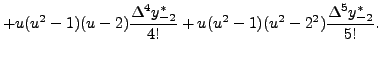
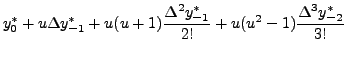
![$\displaystyle y_{0}^*+u\frac{\Delta y_{-1}^*+\Delta
y_0^*}{2}+u^2\frac{\Delta^2...
...frac {
u(u^2-1)}{2}\left[\frac{\Delta^3 y_{-2}^*+\Delta^3 y_{-1}^*
}{3!}\right]$](img5331.png)
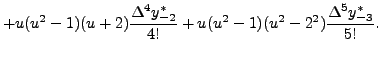
![$\displaystyle + u^2(u^2-1)\frac{\Delta^4 y_{-2}^* }{4!}+
\frac{u(u^2-1)(u^2-2^2)}{2} \left[\frac{\Delta^5 y_{-3}^* +\Delta^5
y_{-2}^*}{5!}\right]+\cdots .$](img5332.png)