Cause and effect for linear systems are related by linear differential equations. note that for the exponential function ![]() ,
,
 |
|
and  |
Consider a function ![]() . If on operation by a system, the function
. If on operation by a system, the function ![]() is only multiplied by a constant
is only multiplied by a constant ![]() , the function is said to be the eigenfunction of the given system, as shown in 8.1.
, the function is said to be the eigenfunction of the given system, as shown in 8.1.
We know that:
 |
(8.1) |
Consider a linear system, as in 8.2. The functions ![]() and
and
![]() are eigen functions of the linear system. If sum of these two
functions is input to the system, the output can be predicted easily,
by superposition theorm. Thus knowing the output to eigenfunctions
helps us in predicting output of several other functions.
are eigen functions of the linear system. If sum of these two
functions is input to the system, the output can be predicted easily,
by superposition theorm. Thus knowing the output to eigenfunctions
helps us in predicting output of several other functions.
Now we look at how output to sinusoidal excitations of linear circuits
can be determined. Consider
![]() or
or
![]() .
.
Note that
![]() . Thus, the phase and associated constant
changes when a sinusoid is passed through a differentiator.
. Thus, the phase and associated constant
changes when a sinusoid is passed through a differentiator.
Similarly,
![]() .
.
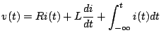
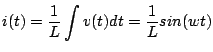
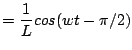
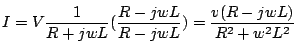
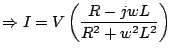
Now consider the RLC circuit shown in 8.3.
 |
|
| If i(t) is sinusoidal, say cos(wt), then | |
 |
|
 |
|
 |
|
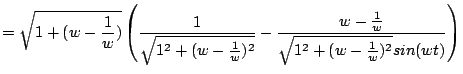
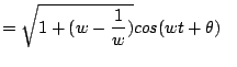 where, where, 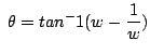 |
![]()
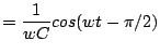
![]() , as shown in 8.4.
, as shown in 8.4.
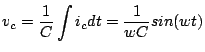
Analysis can be done simply using sin and cos terms.
But can't be further simplified using imaginary quantities
![]()
As in the diagram shown in 8.5,
![]() In figure 8.6, the complex values shown are rotating with time. The
actual value at any time is the projection on the real axis.
In figure 8.6, the complex values shown are rotating with time. The
actual value at any time is the projection on the real axis.
Note that ![]() and
and ![]() have constant separation with each
other. All entities in general will have same relative separation.
have constant separation with each
other. All entities in general will have same relative separation.
Consider figure 8.7. Let us rotate the frame of reference (or
axis) also with speed ![]() rad/sec. Then the angles of
rad/sec. Then the angles of ![]() and
and ![]() with respect to the axis become constants. The figure 8.7 is a
phasor diagram, showing current and voltage phasors, and the phase
difference between the two.
with respect to the axis become constants. The figure 8.7 is a
phasor diagram, showing current and voltage phasors, and the phase
difference between the two.
We show the application of phasors in circuit analysis by the circuit shown in figure 8.8, a simple inductor circuit excited by a sinusoidal voltage source.
 |
|
 |
|
 |
Similarly, consider a resistance excited by a sinusoidal votage
source, as shown in figure 8.10. Here,
![]() , and
, and
![]() is in phase with the
voltage. The same is shown in the phasor diagram 8.11.
is in phase with the
voltage. The same is shown in the phasor diagram 8.11.
Now consider a resistor and an inductor in series with an AC voltage source, as in 8.12.
where 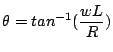 |
The resulting phasor diagram is plotted in figure 8.13.
This gives an inkling to a general result: phasors can be added/subtracted just like vectors. Resulting magnitude and phase would come out to be the same. See the hint below.
In phasor terms: Voltage across inductor: ![]() , Voltage across
resistor
, Voltage across
resistor![]() . Now adding the two vectors,
. Now adding the two vectors,
![]()
Compairing with Ohm's law, ![]() , the previous equation
, the previous equation
![]() ,
the complex term
,
the complex term ![]() can be taken to be similar to resitance. This
is called impedance. Inverse of impedance is called
admittance, complex analog of conductance. In the above
circuit,
can be taken to be similar to resitance. This
is called impedance. Inverse of impedance is called
admittance, complex analog of conductance. In the above
circuit,
 |
|
 |
Similar to the above analysis, we now work with the capacitor. See figure 8.14.
 |
|
 |
Now we analyse circuit shown in in figure 8.16,
![]() . We wish to calculate
. We wish to calculate ![]() and
and ![]() .
.
for first loop: 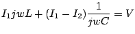 ...(*) ...(*) |
|
for second loop: 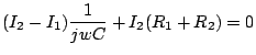 ...(**) ...(**) |
|
From (**): 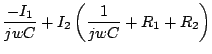 From (*) : From (*) :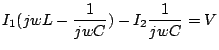 |
Solving these two for ![]() and
and ![]() , we get:
, we get:
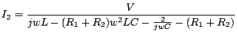 |
|||
| which after rationalization, gives: | |||
 |
For sinusoidal forcing functions, we can use the same techniques, but with complex variables
A sinusoid ![]() passed through a linear system with transfer
function
passed through a linear system with transfer
function ![]() , the output would be
, the output would be
![]() .
.
Thus, for a sum of sinusoids of different frequencies, using
superposition principle, the output for
![]() would be:
would be:
| (8.2) |
![\includegraphics[width=2.0in]{lec7figs/1.eps}](img489.png)
![\includegraphics[width=2.0in]{lec7figs/3.eps}](img500.png)
![\includegraphics[width=2.0in]{lec7figs/4.eps}](img510.png)
![\includegraphics[width=2.0in]{lec7figs/5.eps}](img512.png)
![\includegraphics[width=2.0in]{lec7figs/6.eps}](img514.png)
![\includegraphics[width=2.0in]{lec7figs/7.eps}](img515.png)
![\includegraphics[width=2.0in]{lec7figs/8.eps}](img517.png)
![\includegraphics[width=2.0in]{lec7figs/9.eps}](img523.png)
![\includegraphics[width=2.0in]{lec7figs/10.eps}](img524.png)
![\includegraphics[width=2.0in]{lec7figs/11.eps}](img527.png)
![\includegraphics[width=2.0in]{lec7figs/12.eps}](img528.png)
![\includegraphics[width=2.0in]{lec7figs/13.eps}](img538.png)
![\includegraphics[width=2.0in]{lec7figs/14.eps}](img553.png)
![\includegraphics[width=2.0in]{lec7figs/16.eps}](img554.png)
![\includegraphics[width=2.0in]{lec7figs/15.eps}](img555.png)