


Next: R-C Circuits
Up: Introduction to Electronics
Previous: Using Norton's equivalent
Contents
Figure 6.1:
non-realistic model
|
|
Figure 6.2:
Switch attached to make it realistic
|
|
Figure 6.3:
Inductance of wire also considered
|
|
Figure 6.4:
After closing the switch
|
|
For DC circuit analysis, the voltage and current source excitation is
constant, so C and L are neglected 6.1. The circuit is assumed to
be as it is
since time= to
to  . In practice, no excitation is constant
from
. In practice, no excitation is constant
from  to
to  . A
more realistic circuit would include a switch, as shown in
Fig.6.2. Also, inductance and capacitances of wires and components
cannot be neglected as shown in Fig.6.3, and in Fig.6.4 (for
. A
more realistic circuit would include a switch, as shown in
Fig.6.2. Also, inductance and capacitances of wires and components
cannot be neglected as shown in Fig.6.3, and in Fig.6.4 (for
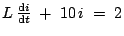
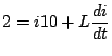
 ). Using KVL:
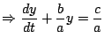
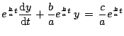
Multiplying both sides by
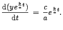
to get
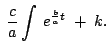
Therefore,
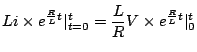
Integrating both sides, we get
Note that, at
 ,
,
 and at
  ,
,
 .
.
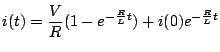
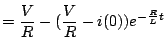
Now,
 , where,
 ,
,  and
and  .
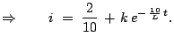
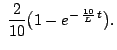
As at
.
As at  ,
,  ,
,
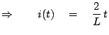
The plot of  vs.
vs.  is shown in the Fig.6.5. Note that when
,
is shown in the Fig.6.5. Note that when
,
 A.
A.
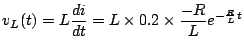
Voltage across the inductor is given by
 . Therefore,
The plot of
. Therefore,
The plot of  vs is shown in Fig.6.6.
From the above equation, we notice that in time
vs is shown in Fig.6.6.
From the above equation, we notice that in time
 seconds,
the voltage across the inductor would reduce to
seconds,
the voltage across the inductor would reduce to
 of its
original value and would go on decreasing by a further factor of
every
seconds thereafter. Therefore,
summing it up, we have for an inductor-resistor pair with a constant
voltage applied at
of its
original value and would go on decreasing by a further factor of
every
seconds thereafter. Therefore,
summing it up, we have for an inductor-resistor pair with a constant
voltage applied at  ,
,
Now, consider the circuit shown in Fig.6.7.
Before , we have the circuit looking as in
Fig.![[*]](crossref.png) . Therefore we have the initial current (at ) through the inductor as
. Therefore we have the initial current (at ) through the inductor as  A.
A.
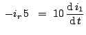
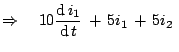
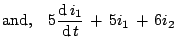
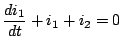
At  , the circuit looks as in Fig. and therefore, we have the following equations for
  .
.
At ,
 A. Hence,
The plot for vs would therefore be as in Fig 5.10
A. Hence,
The plot for vs would therefore be as in Fig 5.10
Figure 6.10:
![\includegraphics[width=3.0in]{lec5figs/10.eps}](img344.png) |
Figure 6.11:
R

![\includegraphics[width=3.0in]{lec5figs/11.eps}](img345.png) |
Hence,
 and, as shown in 6.11, discharge
will be immediate. We write equations for
and, as shown in 6.11, discharge
will be immediate. We write equations for  across the
inductor.
across the
inductor.
Figure 6.12:
Note the sign of
![\includegraphics[width=3.0in]{lec5figs/12.eps}](img349.png) |
Sign of is as shown in 6.12. As
 ,
,
Figure 6.13:
Large inductance doesn't allow currents to change at fast rates
![\includegraphics[width=3.0in]{lec5figs/13.eps}](img352.png) |
Switching off causes a discharge in the tube or spark at switch 6.13.
Figure 6.14:
![\includegraphics[width=3.0in]{lec5figs/14.eps}](img353.png) |
At ,  6.14
6.14
In generic form,
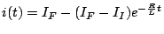
Figure 6.15:
![\includegraphics[width=3.0in]{lec5figs/15.eps}](img360.png) |
Now, have a look at the circuit shown in the figure 5.15. As the resistance  is 0, the
  equations are indeterminate and are of the form
So, we solve the circuit directly
equations are indeterminate and are of the form
So, we solve the circuit directly
At , , therefore, 
We will use the above circuit to analyse the circuit shown in Figure 5.16. As the resistance of  is in parallel with the voltage source and also the rest of the circuit, the current drawn by it will be constant and will not affect the analysis of the rest of the circuit. So, for
 , we can consider the circuit to be as in Figure 5.17. Analysing it as in the previous example, we get
Figure 6.16:
![\includegraphics[width=3.0in]{lec5figs/18.eps}](img375.png) |
Further, for
 , the circuit can be equivalently considered as in Figure 5.19. Notice that still,
  Amps. as the inductor
  is in parallel with the voltage source. The plot for vs. would therefore be linear as in Figure 5.18. Therefore,
Figure 6.17:
![\includegraphics[width=3.0in]{lec5figs/19.eps}](img387.png) |
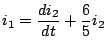
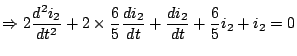
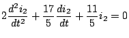
After  , the circuit can be considered equivalently to be that in Fig 5.20. Now, there is no constant voltage source across the resistance of . This, the current flowing through it also comes into the analysis.
Figure 6.18:
![\includegraphics[width=3.0in]{lec5figs/20.eps}](img389.png) |
The solution thus is:
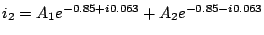 , where, given the
initial conditions, we can solve for
, where, given the
initial conditions, we can solve for  and
and  .
.
Next: R-C Circuits
Up: Introduction to Electronics
Previous: Using Norton's equivalent
Contents
ynsingh
2007-07-25


![\includegraphics[width=3.0in]{lec5figs/1.eps}](img271.png)
![\includegraphics[width=3.0in]{lec5figs/2.eps}](img272.png)
![\includegraphics[width=3.0in]{lec5figs/3.eps}](img273.png)
![\includegraphics[width=3.0in]{lec5figs/4.eps}](img274.png)
![\includegraphics[width=3.0in]{lec5figs/5.eps}](img314.png)
![\includegraphics[width=3.0in]{lec5figs/6.eps}](img318.png)
![\includegraphics[width=3.0in]{lec5figs/7.eps}](img327.png)
![\includegraphics[width=3.0in]{lec5figs/8.eps}](img329.png)
![\includegraphics[width=3.0in]{lec5figs/9.eps}](img330.png)