Major advantages

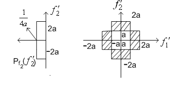
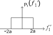
Example 2: Vector quantisation can also exploit non linear dependence. Consider two random variables f₁ and f₂ whose joint pdf is shown in Figure (3.4.6). The pdf is uniform with amplitude 1/(8a²) in the shaded region and '0' outside the shaded region. The marginal density functions and are also shown.

Figure( 3.4.6)

From the joint .

.This implies f₁ and f₂ are linearly independent. However

Therefore f₁ and f₂ are statistically dependent. When the random variables are linearly independent and statistically dependent, they are said to be nonlinearly dependent. If we quantise f₁ and f₂ separately, using the MSE criterion, and allow two reconstruction levels for each of f₁ and f₂, the optimal reconstruction levels for each scalar are 'a' and -a.

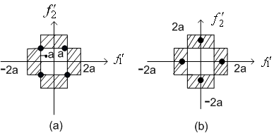
The average distortion is a²/2.

The resulting reconstruction levels in this case are the four filled-in dots shown in Figure(3.4.7).

Figure (3.4.7)

Using vector quantisation, we can choose the four reconstruction levels as shown in    Figure ( 3.4.7). The average distortion D=5a²/12.This example shows that using vector quantisation can reduce the MSE without increasing the number of reconstruction levels.

Linear transformation can always eliminate linear dependence. The nonlinear dependence can be eliminated using an invertible nonlinear operation. If we eliminate linear or non linear dependence prior to quantization, then the advantage that vector quantisation derives from exploiting linear or non linear dependence will disappear.