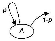
Consider a Discrete Time Markov Chain which is currently in state A. Let p be the probability that the system remains in state A at the next time instant and (1-p) is the probability that it goes to some other state. This may be represented by the figure shown below.

Discrete Time Markov Chain (Transition from State A)

We can then find the probability of the system staying in state A for N time units before exiting from state A as follows -

P{system stays in state A for N time units | given that the system is currently in state A} = p^N

P{system stays in state A for N time units before exiting from state A} = p^N (1-p)

Note that the above distribution is Geometric, which is also memoryless in nature.

Similarly, consider a Continuous Time Markov Chain which is in state A at time t. Let μ be the rate at which the system leaves state A so that the probability of its leaving state A in time interval Δt is μΔt. Then (1-μΔt) will be the probability that the system remains in state A at the time instant t+Δt.

This may be represented by the figure shown below.

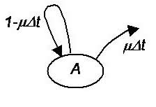
Continuous Time Markov Chain (Transition from State A)

We can then find the probability of the system staying in state A for a time interval of length T units before exiting from state A as follows -

P{system in state A for time T | system currently in state A} = (1 - μΔt )^{T /Δt} → e^{- μT} for Δt → 0
Note that this is the complement of the cumulative distribution function of an exponential distribution implying that the time spent in a particular state (say state A) will be an exponentially distributed random variable.

Note that this distribution is Exponential, which is also memoryless in nature.