

Contents
THE RADIO TELESCOPE AS A SYSTEM
The first system we take for analysis is a simple radio antenna. We examine the antenna
in terms of the system properties looking at them from a radio astronomy perspective. Radio
telescopes are different from conventional idea of Telescope it is actually a standard (and
sometimes a non-conventional) radio antenna. In this sense, we can also say that the radio
telescope dose not directly form an images, as does an optical telescope.
When an optical telescope takes an image, it is collecting rays from specific directions in
the sky and each pixel stores information only about the light it received we cannot get any
details about the pattern within the pixel.
In case of radio telescopes, however, the beam is not as directional as is the case for
optical telescopes. Also, we can say that there is a single pixel or detector in most radio
telescope antennas. (There are some notable exceptions where multiple detectors are put around
the primary focus of parabolic antennas).
Before we go into more details, let us formalize the radio telescope as a system under
consideration. The input to the system is a function of time and some space coordinates.
Typically the space coordinates are the spherical polar coordinates theta and phi. The output of
the system is a plot of the variation of the intensity as a function of some linear coordinate, say
the x axis. If we are imaging a part of the sky rather than a point source, the output may be plotted
as a contour map on the x-y plane, at some given instant of time. Here it is worth noting that since
practically we cannot measure the intensity of all the points at once, such maps are plotted only
for sources where the intensity is not a function of time, or is constant over the time scales
involved in imaging the object.
This system is then seen to have the following properties:
1. Linearity: The system is linear [upto the practical limit of saturation of detectors, this limit is
never attained in practice.]
2. Shift invariance: The system is shift invariant in time i.e. whether we image a steady
source now or later, the output recorded is the same. We note that the system as it stands is
NOT shift invariant in space [as has been discussed above the magnitude of response
recoded depends on where the object is. More on this is discussed below]. However, if we
tracking the source, the coordinate frame is with respect to the principal axis of the telescope.
In that case, we see that the system is shift invariant in space also but this interpretation is
open to discussion, or to be more precise, depends on the convention adopted.
3. Stability: The system is stable. This is rather intuitive, as no practical system can ever give
an unbounded output limiting factors will always take it to a saturation level. We can talk of
this in slightly more formal terms by noting that given an input x(t) to the system, the output
y(t) can be obtained by kx(t) where k is an appropriate constant with dimensions. Then we
can see that if x(t) is bounded, y(t) is also bounded.
4. Causality: The system is causal. Although we will later see that there is a convolution
involved, it is not looking into the future it is a convolution in the space coordinates. The
output of the system at any given time depends only on the input at that instant. Here we are
neglecting the tiny processing delays that may creep in. In that case, the system just adds a
constant delay, but still remains causal.
5. Memory: The antenna and detector by themselves are memory-less. They take the input of
radio waves, and give the corresponding output. All operations are point-by-point. However,
if we record the output on any device which we consider to be a part of the system, it can be
said to have memory. Again, this is a limited version of memory, as the output variable is not
dependent on time, but is dependent on another quantity (say the x variable) proportional to
time.
6. Invertibility: The system is not invertible. Although it is linear and one-one in mapping the
input to the output, we cannot expect the telescope to emit radio waves given the graph
plotted at the output. However, if we feed in electrical signals to the antennas, they are
capable of radiating radio waves. We do not make a general statement here about whether
this system with radio waves incident on the antenna and some electrical signal as output, is
invertible or not. There are several factors which come into play here before we get the output
signal, and the system still need not be invertible.
Now, having taken a look at the basic system properties, let us consider an antenna
observing something in the sky. Had we been talking of an optical telescope, we would have said
that the telescope being pointed in a certain direction, is taking an image of the sky in that
direction. The case of a radio telescope, however, is different: the antenna does not have such a
narrow beam. The antenna responds to radiation coming from different directions. We can
arbitrarily fix the maximum response of the antenna as unity and plot the response in different
directions on an r-theta plot. A typical such plot is given below:
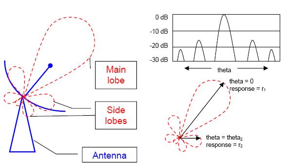
We see that the response plotted in r-theta shows lobes the r is the fraction of
incident radiation along that direction that the antenna would detect. The direction along which
the response is unity is called the principle axis. This is usually normal to the antenna. The
coordinate theta (or phi, as the case may be) is measured with respect to this axis.
On the right we have plotted the antenna response or the so called lobe pattern on an xy
graph: the angle theta is plotted on the x axis, while on the y axis we plot the response of the
antenna to radiation form that direction, in decibels. The response of the antenna is the total
amount of radiation coming from the sky. Here, we note that the antenna can give the same
response to several possible sources: as an example, we see that the antenna would give the same
output for a source of intensity k/r1 along the principle axis, as for a source of intensity k/r2 along
the direction theta2 shown in the figure.
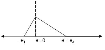
Now we take a look at how a radio telescope images the sky. Instead of considering the
realistic lobe pattern depicted above, let us take up a simplified lobe pattern for analysis. This
pattern is shown below with theta (measured from the principle axis) plotted on the horizontal
axis and intensity plotted on the vertical axis.
Now, let us consider the antenna sweeping across a point source what we see on the
graph is as follows:
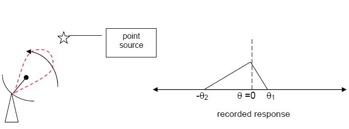
Notice that we have the recorded impulse as some sort of an impulse response of the
system. Since we are talking of an LSI system, this impulse response characterizes the system
completely. So, if we have an extended source in the sky, and the antenna sweeps over it, what
we record is the convolution of the source with the antenna lobe pattern. This is illustrated in the
figure below:
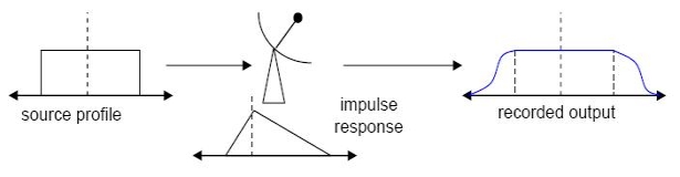
Using this output, we can reconstruct the source profile if we know the lobe pattern
(impulse response) of our antenna.
Here, we shift our attention to a more advanced technique of studying radio sources
interferometry.

