(4) Obtaining distribution functions of left going and right going electrons:
Let us now consider that the bias voltage, V, is applied and the Fermi level of the ferromagnetic lead is shifted by eV, then the distribution function of right-going electrons is given by
(28) |
Where fo is the Fermi-Dirac distribution function. Similarly, the distribution function of the left-going electrons can be defined as
(29) |
(5) Calculating the current:
Substituting eqns.(29) and (28) in eqn.(8), the current flowing through the junctions is obtained as
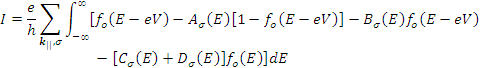 |
(30) |
The probabilities of Cσ(E) and Dσ(E) can be eliminated by using the relation
(31) |
Substituting eqn.(31) in eqn.(30) results
 |
(32) |
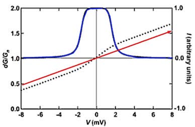
Figure 20.1: Normalized differential conductance (blue curve) and current (dotted curve) versus the bias voltage V of a ballistic (Z = 0) point contact described by BTK model. The curve (red) passing through the origin represents a simple Ohmic case.