6.2 Macroscopic view of Magnetization

We will refer to the same geometry here where we have a current carrying coil.

We define magnetic induction, B, as μ₀H where μ₀ is magnetic permeability of vacuum and its value is equal to 4π * 10^-7H.m^-1 . Units of B are tesla or Weber.m^-2.

This also explains that while H  depends only on the current, B  also depends upon the medium surrounding the wire which defines μ₀.

So now rewriting equation (6.1) yields

(6.10)

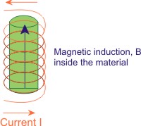
Now imagine if a magnetic material is inserted within the coil, then there is a current induced in the magnetic material too, called Ameprian current, I_a which modifies the equation (6.10) to

(6.11a)

This Amperain current in the magnetic material can be replaced with induced magnetization, M, and hence using Equation (6.11a), we can write

(6.11b)

If magnetization is assumed to be proportional to the magnetizing field, H, with proportionality constant defined as magnetic susceptibility, χ_m i.e. M = χ_m.H,  we can write

(6.12)

Here, χ_m,  similar to dielectric materials, can be thought of as a parameter which expresses magnetic response of electron in a material to the applied magnetic field and is a dimensionless quantity. Here, μ_r = (1+ χ_m) is the, in a similar manner to relative dielectric permittivity, ε_r.

In general, both susceptibility and permeability are tensors and assuming that vectors are collinear wherever there is vector notation is not used.