Formulation of a High Precision Plate Element

The plate elements with lower degree of polynomial displacement functions cannot simulate true curvature distribution precisely unless a very fine mesh is generated. Bending moment or shear stresses generated by such polynomials are discontinuous as inter element continuity cannot be ensured with a low degree polynomial. Also, many engineering laminates are thin and are analyzed using Classical Laminated Plate Theory (CLPT). By virtue of Kirchhoff hypothesis, the model neglects the effects due to transverse shear and normal strain in the thickness direction. The present finite element formulation is based on CLPT and, thus, limited to thin plates. The element has 3 nodes at the vertices and uses 12 degrees of freedom at each vertex, the in plane displacements in the x and y directions and their first derivatives, along with the normal displacement in the thickness direction and its first and second derivatives. Two more in-plane displacements at the centroid of the element are condensed out before assembly. The displacement functions used here are the same as used in the high precision elements developed by Jeyachandrabose et al [1985] and Bhattacharya et al [1998]. These high precision elements are recognized for accurate deformation prediction. They have used complete cubic polynomials for the in-plane displacements u, v and a constrained quintic polynomial for the normal displacement w. The elements are completely conforming and rapidly converging. Each element has total 38 degrees of freedom (DOF). The coordinate system and element configuration are shown in Figure 16.1.

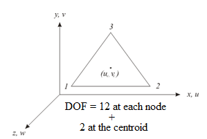
Figure 16.1: Triangular element used in HPFE

Consider the deformation of a laminate in x-z plane and assume that normal to the mid plane remain straight and normal after deformation. This assumption is equivalent to neglecting shearing deformations  and is also equivalent to assuming that the lamina that make up the cross section do not slip over each other.