In another recent investigation (Srinivas et. al., 2006), the locally dynamic SGS model of Piomelli and Liu (1995) is used in order to carry out LES of turbulent flow past a partially enclosed square cylinder. The various integral parameters are presented in Table 35.2 namely, the time- and span-averaged lift and drag coefficients, rms values of the drag and lift coefficients, Strouhal number ( St ), the mean recirculation length ( lr ) and the mean base pressure coefficients (  ). Table 35.2 also compares the results of present simulation with the experimental data and the LES results of Wang and Vanka (1996). It can be observed from Table 35.2 that the present calculated results are in excellent agreement with the experimental data of Lyn et al. (1995) and the LES results of Wang and Vanka (1996). ). Table 35.2 also compares the results of present simulation with the experimental data and the LES results of Wang and Vanka (1996). It can be observed from Table 35.2 that the present calculated results are in excellent agreement with the experimental data of Lyn et al. (1995) and the LES results of Wang and Vanka (1996).
|
Re |

|

|

|

|
St |
lr
|
|
Present Computation |
2.14 × 10⁴ |
0.0 |
1.12 |
2.14 |
0.17 |
0.135 |
1.31 |
1.65 |
Lyn et al. (1995) |
2.14 × 10⁴ |
|
|
2.1 |
|
0.132 |
1.38 |
1.6 |
Wang and Vanka (1996) |
2.14 × 10⁴ |
0.04 |
1.29 |
2.03 |
0.18 |
0.13 |
1.26 |
|
Noda and Nakayama (2003) |
6.89 × 10⁴ |
|
1.180 |
2.164 |
0.207 |
1.131 |
|
1.483 |
Durao et al. (1998) |
1.4 × 10⁴ |
|
|
|
|
0.138 |
1.33 |
|
Lee (1975) |
1.76 × 10⁴ |
|
|
2.05 |
0.23 |
0.122 |
|
1.3 |
Norberg (1993) |
2.2 × 10⁴ |
|
|
2.1 |
|
0.13 |
|
1.37 |
Table 35.2: Integral parameters compared with LES and Experimental Studies
The time-averaged streamwise velocity profiles at different downstream locations ( x = 0.0,1.0,1.5 and x = 5) are presented in Figure 35.4, which shows that the results due to the present computation, in general, are in good agreement with their experimental counterpart. The centerline velocity is negative at the location of ( x = 1.0). The recovery of velocity is directly related to the wake-width, which in turn depends on the entrainment at the edge of the wake. The time averaged streamwise velocity at any point in the wake is smaller than that at the free stream. This entails attenuation of the minimum velocity at the centerline. In the downstream, say at x = 5.0, the average velocity profile is still non-uniform.
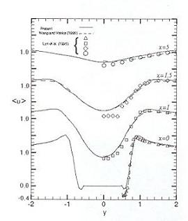
Figure 35.4: The time-averaged streamwise velocity profiles at different downstream locations.
|