Theory of Hydrodynamic Lubrication

• Thin film of oil, confined between the interspace of moving parts, may acquire high pressures up to 100 MPa which is capable of supporting load and reducing friction. The salient features of this type of motion can be understood from a study of slipper bearing (Fig. 27.2). The slipper moves with a constant velocity U past the bearing plate. This slipper face and the bearing plate are not parallel but slightly inclined at an angle of . A typical bearing has a gap width of 0.025 mm or less, and the convergence between the walls may be of the order of 1/5000. It is assumed that the sliding surfaces are very large in transverse direction so that the problem can be considered two-dimensional.

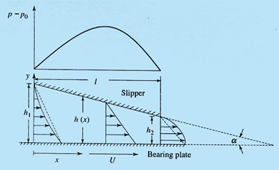
Fig 27.2 - Flow in a slipper bearing

• For the analysis, we may assume that the slipper is at rest and the plate is forced to move with a constant velocity U .
• The height h(x) of the wedge between the block and the guide is assumed to be very small as compared with the length l of the block.
• The essential difference between this motion and that discussed in Lecture 26 (Couette flow) is that here the two walls are inclined at an angle to each other.
• Due to the gradual reduction of narrowing passage, the convective acceleration is distinctly not zero.
• For all practical purposes, inertia terms can be neglected as compared to viscous term. This can be justified in following way

The inertia force can be neglected with respect to viscous force if the modified Reynolds number,

• The equation for motion in y direction can be omitted since the v component of velocity is very small with respect to u . Besides, in the x-momentum equation, can be neglected as compared with because the former is smaller than the latter by a factor of the order of . With these simplifications the equations of motion reduce to

(27.6)

The equation of continuity can be written as :

(27.7)

The boundary conditions are:
at y = 0, u = U at x = 0, p = p₀
at y = h, u = 0 and at x = l, p = p₀                                                                 (27.8)

• Integrating Eq. (27.6) with respect to y , we obtain

• Application of the kinematic boundary conditions (at y=0, u =U and y = h, U=0), yields

(27.9)

Note that is constant as far as integration along y is concerned, but p and vary along x -axis.

• At the point of maximum pressure, =0 hence

(27.10)

• Equation (27.10) depicts that the velocity profile along y is linear at the location of maximum pressure. The gap at this location may be denoted as h^*.
• Substituting Eq. (27.9) into Eq. (27.8) and integrating, we get

or

(27.11)

where

• Integrating Eq. (27.11) with respect to x , we obtain

(27.12a)

or

(27.12b)

where    is a constant

• Since the pressure must be the same (p = p₀), at the ends of the bearing, namely, p = p₀ at x = 0 and p = p₀ at x=l, the unknowns in the above equations can be determined by applying the pressure boundary conditions. We obtain

• With these values inserted, the equation for pressure distribution (27.12) becomes

or	(27.13)

• It may be seen from Eq. (27.13) that, if the gap is uniform, i.e. h = h₁=h₂, the gauge pressure will be zero. Furthermore, it can be said that very high pressure can be developed by keeping the film thickness very small.
• Figure 27.2 shows the distribution of pressure throughout the bearing.