Weighted Residual Method
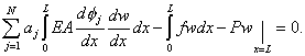
In this method, we use the integral form corresponding to the weighted residual formulation (equation 2.5b) while obtaining an approximate solution. We rearrange equation (2.5b) as follows :
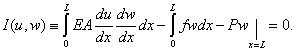 | | |
(3.68) |
As in the Ritz method, an approximate solution is assumed as a series of N terms involving the unknown coefficients  and a set of linearly independent functions and a set of linearly independent functions  defined over the interval [0,L] : defined over the interval [0,L] :
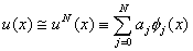 |
(3.69) |
The application of the Dirichlet boundary condition on  (equation 2.1b) to this expression leads to (equation 2.1b) to this expression leads to
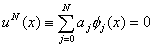 at at  |
(3.70) |
If we assume that all  except except  satisfy the condition satisfy the condition
 at at  |
(3.71) |
then, from equation (3.70), we get
 |
(3.72) |
Then, the expression (3.69) starts from i = 1 rather then from i = 0. Thus,
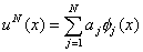 |
(3.73) |
Substitution of this expression in equation (3.68) leads to :
 |
(3.74) |
To convert the above equation into a set of N algebraic equations in the unknown coefficients  , we choose N weight functions as follows : , we choose N weight functions as follows :
 |
for  |
(3.75) |
Here, the functions  represent another set of linearly independent functions defined over the interval [0, L ]. Note that the functions represent another set of linearly independent functions defined over the interval [0, L ]. Note that the functions  must satisfy the constraints arising out of the admissibility conditions of the weight function must satisfy the constraints arising out of the admissibility conditions of the weight function  . These conditions are stated in section 2.2. . These conditions are stated in section 2.2.
When the functions  are different from are different from  , the corresponding weighted residual method is called as the Petrov-Galerkin Method. On the other hand, when the functions , the corresponding weighted residual method is called as the Petrov-Galerkin Method. On the other hand, when the functions  are the same as are the same as  , then the method is called as the Galerkin Method. The next section describes the details of the Galerkin method. , then the method is called as the Galerkin Method. The next section describes the details of the Galerkin method.
|