Higher Order Lagrangian Rectangular Elements

Note that the approximating function for the simplest rectangular element (eq. 24.1) is not a complete polynomial, and hence does not satisfy the property of spatial invariance or geometric isotropy. Thus, its form does not become independent of the orientation of the coordinate system. However, when we use rectangular elements, the domain is rectangular and, therefore, the orientation of the coordinate system is almost fixed (Fig. 25.1a). The only other possible orientation is to interchange x and y axes (Fig. 25.1b).

Figure 25.1 Choice of (x, y) Axes for Rectangular Element

Therefore, the form of the approximating function for rectangular elements need not satisfy the property of spatial invariance exactly but need to satisfy only the following restricted version : The form of the approximating function should be symmetric in x and y coordinates. (If the approximating function is expressed in terms of the natural coordinates then it should be symmetric in and coordinates). To satisfy the restricted version of the spatial isotropy, the approximating function must contain :

• the terms on the axis of the symmetry of the Pascal Triangle (Fig. 23.1) and/or,
• equal number of symmetrically placed terms form each side of the Pascal Triangle (Fig. 23.1).

As in the case of higher order triangular elements (Lecture 23), here also we construct the shape functions directly in terms of the natural coordinates. Therefore, we start with the approximating function expressed in terms of the natural coordinates of . To satisfy the restricted version of spatial isotropy, we choose the approximating function to be a product of 1-D polynomial in and 1-D polynomial in , both being of the same degree. Thus, p -th order Lagrangian approximation is constructed by using the product of p -th degree 1-D polynomial in and p -th degree 1-D polynomial in . Note that the approximating function (eq. 24.6) of the simplest rectangular can be expressed as the product of 1 st degree 1-D polynomial in and 1 st degree 1-D polynomial in . Therefore, it is consistent to call it as the 1 st order ( p =1) Lagrangian approximation. Note that p -th order Lagrangian approximation contains all the terms which fall within p -th parallelogram of the Pascal Triangle in shown in Fig. 25.2.

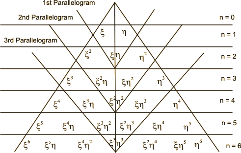
Figure 25.2 Pascal Triangle in Natural Coordinates

As in the case of higher order Lagrangian triangular elements (Lecture 23), here also, the number of nodes per element ( N ) must be equal to the number of coefficients in the approximating function. Therefore

(25.1)

As stated in Lecture 23, for the weighted residual integral to be finite, the approximating function must be such that the primary variable is continuous across the inter-element boundaries. For rectangular elements, the boundaries of the master element are and . Since, the approximating function is a product of p -th degree 1-D polynomial in and p -th degree 1-D polynomial in , the variation of the primary variable along any boundary becomes a p -th degree 1-D polynomial in the boundary coordinate. To make the primary variable continuous across the inter element boundaries, its variation along the common boundary segment must be the same as that of the adjoining element. For this to happen, the number of nodes (which is equal to the degrees of freedom) on the common boundary segment must be equal to ( p +1). Since the rectangular element has four boundary segments, the number of boundary nodes becomes

(25.2)

Since 4 nodes are common to 4 pairs of boundaries, they must be subtracted from 4( p +1) to get the number of boundary nodes N_b . The remaining nodes must be in the interior of the element. Thus, the number of internal nodes is given by :

(25.3)

For p = 1, i.e., for the first order or bi-linear approximation in and , as per equations (25.1)- (25.3), the number of various nodes is . Similarly, for p = 2, i.e., for the second order or bi-quadratic approximation in and , the number of various nodes is . Thus, there is one internal node. Similarly, for p = 3, i.e., for the third order or bi-cubic approximation in and , the number of various nodes is N = 16 , N_b = 12, N_i = 4 . Thus, there are 4 internal nodes.