Model Boundary Value Problem

To illustrate the development of integral formulations, the following model boundary value problem is considered. It represents the axial extension (or compression) of a bar shown in Fig. 2.1.

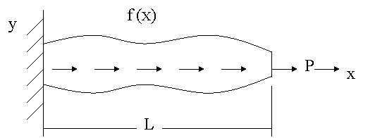
Figure 2.1

The bar has a variable area of cross-section which is denoted by the function A(x). The length of the bar is L. The Young's modules of the bar material is E . The bar is fixed at the end x = 0. The forces acting on the bar are (i) a distributed force f(x), which varies with x and (ii) a point force P at the end x = L . The axial displacement of a cross-section at x, denoted by u(x), is governed by the following boundary value problem consisting of a differential equation (DE) and two boundary conditions (BC):

DE:		0<x<L	(2.1a)
BC:	(i)  u = 0	at x=0	(2.1b)
	(ii) EA(x)	at x=L	(2.1c)

The differential equation represents the equilibrium of a small element of the bar expressed in terms of the displacement using the stress-strain and strain-displacement relations. The boundary condition (2.1b) is a geometric or kinematic boundary condition. Since, it is a condition on the primary variable u(x), it is called as Dirichlet boundary condition. The second boundary condition (condition 1c) is a force boundary condition, or a condition on the secondary variable (i.e., axial force). Since, it is a condition on a derivative of the primary variable; it is called as the Neumann boundary condition.