CONVOLUTION BACK-PROJECTION

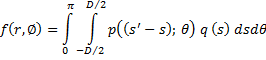
In the convolution back-projection algorithm (CBP), the reconstructed function,, is evaluated by the integral formula

where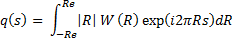

Here is the projection data and is the perpendicular distance of the data ray from the center of the object. In addition, denotes the source-detector line with respect to a fixed axis (and hence the view angle), is the diameter of the growth chamber, and s’ is the s-value of the data ray passing through the point . The symbol is the Fourier frequency, is the convolving function of Equation 5, and is the filter function. Also see Figure 5.16 for an explanation on the notation used. The filter function vanishes outside the interval and is an even function of . Here is the Fourier cut-off frequency and is taken to be being the ray spacing. The reconstruction obtained is specific to the choice of the filter function A Hamming filter h 54 has been used in the present study. For it is given by the formula

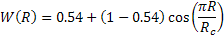
This filter emphasizes the smooth features of the concentration variation, while suppressing small-scale (fine structure) fluctuations. This is quite appropriate to the present study for the following reason. Density variations in the solution arise primarily because of the deposition of the solute on the growing faces of the crystal as the solution is cooled at a given rate. Since the crystal growth rate is slow, one encounters density variations that are distributed in the entire solution, while rapid fluctuations in concentration do not appear. Hence, it is of interest to reconstruct the dominant pattern in the concentration field rather than its secondary features.