Curve Fitting Approach

In this method, the intensity minima are assumed to coincide with the center of the fringe bands. Specifically, the variations in the grey levels are not made use of. This is equivalent to the classical microscope route of fringe analysis. A few points within each band are collected using a pixel viewing utility available on workstations. The number of points to be collected over an entire fringe depends on the nature of the function to be fitted through the fringe curve. A greater number of points is chosen in the region of sharp changes in the fringe slope. Relatively fewer points are chosen when the fringe shape varies uniformly or is a constant. In the present work, a cubic spline has been fitted through sets of four points while maintaining slope continuity between adjacent data sets. While this methods has the disadvantages of not identifying the minimum intensity location, it does offer certain advantages. These are, thinning of all fringes with no loss and smoothness of the fringe skeleton.

 Figure 4.22 shows the thinned images obtained using the curve fitting approach corresponding to the interferograms in Figure 4.20. In the Interferograms for the 90 degree projection, an extra fringe can be seen to be captured. This could not be resolved using the automatic fringe thinning approach. Figure 4.23 shows the thinned images superimposed with the original interferograms. The match is again seen to be good.

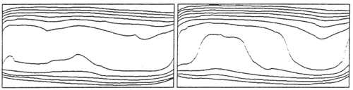
Figure 4.22: Thinned images, 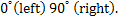curve fitting method for fringe thinning

Figure 4.23: Superimposed thinned images (curve fitting method) with original images,