The boundaries of the image, i.e. the window size are to prescribed as an input to the computer code. On reaching the boundary, control in the computer code is transferred to the starting points so that the rest of the fringe in the opposite direction can be traced. The algorithm used for fringe tracing is summarized below:

1. Initialize the thinned image as black (intensity 0).
2. Read the image containing the interferogram including the boundary.
3.  Read the starting point data for all the fringes in the image. These points can lie the interior of the image.
4. Specify the desired template size at the starting point.
5. Specify the initial direction of movement to the left or right.
6. Obtain the intensity sums in the eight directions and find the two minima.
7. Start tracing in the direction of the minimum intensity.
8. At the boundary, transfer control to starting point.
9. Start tracing in the opposite direction until the boundary is reached.
10. Assign a grey level of 225 to the traced pixels.
11. Repeat the process for all the fringes.

Figure 4.20 shows the thinned image developed using the procedure given above. Both zero and 90 degree projections are shown.

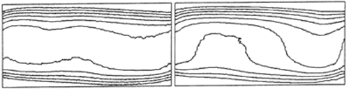
Figure 4.20: Thinned images, 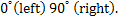,automatic fringe thining

Figure 4.21 shows the superposition of the fringe skeleton and the interferograms and the agreement can be seen to be satisfactory. The fringe immediately adjacent to the top wall could not be resolved in the sense that a minimum intensity direction could not be identified in certain parts of the image. This could have been taken care of by manually joining the two segments of the fringe. Instead, the unresolved fringe has been deliberately taken to be lost. As discussed later, this was not seen to introduce error in the tomographically reconstructed temperature field. A closer evaluation of the thinning process is taken up in section 4.2

Figure 4.21: Superimposed thinned images (automatic fringe thinning) with original images,