The linearized system (10.44) thus reads
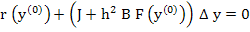 |
(10.47) |
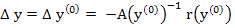
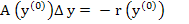
and its solution is given by
provided that the inverse of the matrix
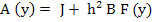
exists for  . If all goes well, the vector . If all goes well, the vector 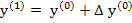 will be a better approximation to the exact solution, the residual vector will be a better approximation to the exact solution, the residual vector  will be smaller, and the process will be smaller, and the process
can be repeated with  taking the place of taking the place of  , etc. until the convergence is achieved. Since for problems of class M, the system (10.44) has a unique solution , etc. until the convergence is achieved. Since for problems of class M, the system (10.44) has a unique solution  for sufficiently small values of for sufficiently small values of  , and it is known that Newton's method produces a sequence of vectors , and it is known that Newton's method produces a sequence of vectors  which converges rapidly to provided that the initial approximation is not too bad. Here we are mainly concerned with the question of computational technique. In this respect it should be noted that for the solution of (10.47) it is not necessary to calculate the inverse of the matrix which converges rapidly to provided that the initial approximation is not too bad. Here we are mainly concerned with the question of computational technique. In this respect it should be noted that for the solution of (10.47) it is not necessary to calculate the inverse of the matrix  . All that is required is the solution of the system of linear equations . All that is required is the solution of the system of linear equations
For the components of  . This solution is greatly facilitated by the fact that the matrix is again tri-diagonal. In fact, if . This solution is greatly facilitated by the fact that the matrix is again tri-diagonal. In fact, if  , we have , we have


and all other elements are zero.
The method described for the linear case thus is immediately applicable. The only work that is required for one step of Newton's method in addition to the work involved in the solution of a linear system is the evaluation of the residual vector  and of the partial derivative and of the partial derivative  (n = 1, 2, … , N -1). (n = 1, 2, … , N -1). |
|