1 Performance Indices
Whenever we use the term optimal to describe the effectiveness of a given control strategy, we do so with respect to some performance measure or index.
We generally assume that the value of the performance index decreases with the quality of the control law.
Constructing a performance index can be considered as a part of the system modeling. We would now discuss some typical performance indices which are popularly used.
Let us first consider the following system
![]()
![]()
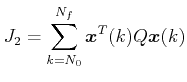
Suppose that the objective is to control the system such that over a fixed interval ![]() , the components of the state vector are as small as possible. A suitable performance to be minimized is
, the components of the state vector are as small as possible. A suitable performance to be minimized is
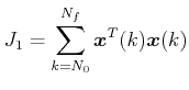
When J1 is very small, ![]() is also very small.
is also very small.
If we want to minimize the output over a fixed interval ![]() , a suitable performance would be
, a suitable performance would be
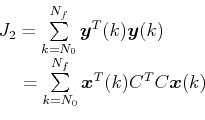
If ![]() , which is a symmetric matrix,
, which is a symmetric matrix,