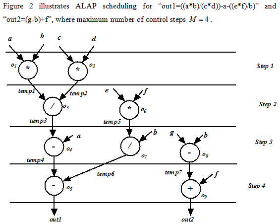
Figure 2. ALAP scheduling for “out1=((a*b)/(c*d))-a-((e*f)/b)” and “out2=(g-b)+f”

In this case, it may be noted that operations 0₅, 0₉ do not have any direct successors, i.e., they generate output values. So these operations have the control step as M=4 . Operation 0₅is the immediate successor of 0₄ , so, control_step(0₅) = control_step(0₅)-1=3. Similarly, control step assignment for all operations can be explained.

This schedule is complete within the 1 st control step, thereby making it successful. The resource requirements are—

Step1: 2 Multipliers
Step2: 1 Dividers + (multiplier from Step1 can be used)
Step3: 2 subtractors + (divider from Step2 can be used)
Step4: 1 adder + (subtractor from Step3 can be used)

If ALAP is compared with ASAP, it may be noted that we have achieved the following.

Saved 1 Multiplier by delaying O₆ from step1 to step2.
Saved 1 Divider by delaying O₇ from step2 to step3.
Increased 1 subtractor by delaying O₈ from step1 to step3.

So, it may be observed that for the subpart of the expression, “(e*f)/b”, ALSP is better compared to ASAP. However, for the expression, “out2=(g-b)+f” ASAP is better compared to ALAP. As already mentioned, ALSP and ASAP are heuristics and may not generate an optimal solution. By applying the scheme ALAP for “(e*f)/b” and ASAP for “out2=(g-b)+f”, the schedule we obtain for M=4 is shown in Figure 3.

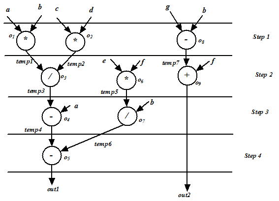
Figure 3. ALAP scheduling for “((e*f)/b)” and ASAP for “out2=(g-b)+f”

It may be noted that the resource consumption in case of Figure 3 is as follows.

Step1: 2 Multipliers + 1 subtractor
Step2: 1 Divider + (multiplier from Step1 can be used) + 1 adder
Step3: 1 subtractors + (subtractor from Step1 can be used) + (divider from Step2 can be used)
Step4: (subtractor from Step3 can be used)

So it may be noted that a schedule which is a “mix of ALAP and ASAP” provides better solution than by the individual algorithms.

In the next section we will see FDS scheduling algorithm which is motivated from above fact of combining ALAP and ASAP.