Worked-out Examples:

Population Forecast by Different Methods
Sedimentation Tank Design
Rapid Sand Filter Design
Flow in Pipes of a Distribution Network by Hardy Cross Method
Trickling Filter Design

Population Forecast by Different Methods

Problem: Predict the population for the years 1981, 1991, 1994, and 2001 from the following census figures of a town by different methods.

Solution:

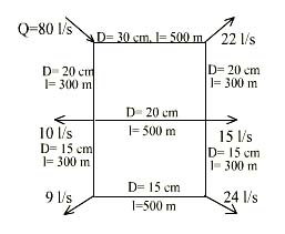
+=increase; - = decrease

Arithmetical Progression Method:

P_n = P + ni

Average increases per decade = i = 8.57

Population for the years,

1981= population 1971 + ni, here n=1 decade

        = 120 + 8.57 = 128.57

1991= population 1971 + ni, here n=2 decade

        = 120 + 2 x 8.57 = 137.14

2001= population 1971 + ni, here n=3 decade

        = 120 + 3 x 8.57 = 145.71

1994= population 1991 + (population 2001 - 1991) x 3/10

        = 137.14 + (8.57) x 3/10 = 139.71

Incremental Increase Method:

Population for the years,

1981= population 1971 + average increase per decade + average incremental increase

        = 120 + 8.57 + 3.0 = 131.57

1991= population 1981 + 11.57

        = 131.57 + 11.57 = 143.14

2001= population 1991 + 11.57

        = 143.14 + 11.57 = 154.71

1994= population 1991 + 11.57 x 3/10

        = 143.14 + 3.47 = 146.61

Geometric Progression Method:

Average percentage increase per decade = 10.66

P _n = P (1+i/100) ⁿ

Population for 1981 = Population 1971 x (1+i/100) ⁿ

= 120 x (1+10.66/100), i = 10.66, n = 1

= 120 x 110.66/100 = 132.8

Population for 1991 = Population 1971 x (1+i/100) ⁿ

= 120 x (1+10.66/100) ² , i = 10.66, n = 2

= 120 x 1.2245 = 146.95

Population for 2001 = Population 1971 x (1+i/100) ⁿ

= 120 x (1+10.66/100) ³ , i = 10.66, n = 3

= 120 x 1.355 = 162.60

Population for 1994 = 146.95 + (15.84 x 3/10) = 151.70

Sedimentation Tank Design

Problem: Design a rectangular sedimentation tank to treat 2.4 million litres of raw water per day. The detention period may be assumed to be 3 hours.

Solution: Raw water flow per day is 2.4 x 10⁶ l. Detention period is 3h.

Volume of tank = Flow x Detention period = 2.4 x 10³ x 3/24 = 300 m³

Assume depth of tank = 3.0 m.

Surface area = 300/3 = 100 m²

L/B = 3 (assumed). L = 3B.

      3B² = 100 m² i.e. B = 5.8 m

       L = 3B = 5.8 X 3 = 17.4 m

Hence surface loading (Overflow rate) = 2.4 x 10⁶ = 24,000 l/d/m² < 40,000 l/d/m² (OK)
                                                                 100

Rapid Sand Filter Design

Problem: Design a rapid sand filter to treat 10 million litres of raw water per day allowing 0.5% of filtered water for backwashing. Half hour per day is used for bakwashing. Assume necessary data.

Solution: Total filtered water = 10.05 x 24 x 10⁶ = 0.42766 Ml / h
                                                    24 x 23.5

Let the rate of filtration be 5000 l / h / m² of bed.

Area of filter = 10.05 x 10⁶ x    1     = 85.5 m²
                           23.5           5000

Provide two units. Each bed area 85.5/2 = 42.77. L/B = 1.3; 1.3B² = 42.77

B = 5.75 m ; L = 5.75 x 1.3 = 7.5 m

Assume depth of sand = 50 to 75 cm.

Underdrainage system:

Total area of holes = 0.2 to 0.5% of bed area.

Assume 0.2% of bed area =  0.2  x 42.77 = 0.086 m²
                                            100

Area of lateral = 2 (Area of holes of lateral)

Area of manifold = 2 (Area of laterals)

So, area of manifold = 4 x area of holes = 4 x 0.086 = 0.344 = 0.35 m² .

 \ Diameter of manifold = (4 x 0.35 /p)^1/2 = 66 cm

Assume c/c of lateral = 30 cm. Total numbers = 7.5/ 0.3 = 25 on either side.

Length of lateral = 5.75/2 - 0.66/2 = 2.545 m.

C.S. area of lateral = 2 x area of perforations per lateral. Take dia of holes = 13 mm

Number of holes:   n p (1.3)² = 0.086 x 10⁴ = 860 cm²
                                4 

      \ n = 4 x 860 = 648, say 650
                p (1.3)²

Number of holes per lateral = 650/50 = 13

Area of perforations per lateral = 13 x p (1.3)² /4 = 17.24 cm²

Spacing of holes = 2.545/13 = 19.5 cm.

C.S. area of lateral = 2 x area of perforations per lateral = 2 x 17.24 = 34.5 cm².

       \ Diameter of lateral = (4 x 34.5/p)^1/2 = 6.63 cm

Check: Length of lateral < 60 d = 60 x 6.63 = 3.98 m. l = 2.545 m (Hence acceptable).

Rising washwater velocity in bed = 50 cm/min.

Washwater discharge per bed = (0.5/60) x 5.75 x 7.5 = 0.36 m³/s.

Velocity of flow through lateral =          0.36          =   0.36 x 10 ⁴ = 2.08 m/s (ok)
                                                  Total lateral area      50 x 34.5

Manifold velocity =    0.36    = 1.04 m/s < 2.25 m/s (ok)
                                0.345

Washwater gutter

Discharge of washwater per bed = 0.36 m³/s. Size of bed = 7.5 x 5.75 m.

Assume 3 troughs running lengthwise at 5.75/3 = 1.9 m c/c.

Discharge of each trough = Q/3 = 0.36/3 = 0.12 m³/s.

              Q =1.71 x b x h^3/2

Assume b =0.3 m

              h^3/2 =    0.12      = 0.234
                       1.71 x 0.3

            \ h = 0.378 m = 37.8 cm = 40 cm

                   = 40 + (free board) 5 cm = 45 cm; slope 1 in 40

Clear water reservoir for backwashing

For 4 h filter capacity, Capacity of tank = 4 x 5000 x 7.5 x 5.75 x 2 = 1725 m³
                                                                              1000

Assume depth d = 5 m. Surface area = 1725/5 = 345 m²

L/B = 2; 2B² = 345; B = 13 m & L = 26 m.

Dia of inlet pipe coming from two filter = 50 cm.

Velocity <0.6 m/s. Diameter of washwater pipe to overhead tank = 67.5 cm.

Air compressor unit = 1000 l of air/ min/ m² bed area.

For 5 min, air required = 1000 x 5 x 7.5 x 5.77 x 2 = 4.32 m³ of air.

Flow in Pipes of a Distribution Network by Hardy Cross Method

Problem: Calculate the head losses and the corrected flows in the various pipes of a distribution network as shown in figure. The diameters and the lengths of the pipes used are given against each pipe. Compute corrected flows after one corrections.

Solution: First of all, the magnitudes as well as the directions of the possible flows in each pipe are assumed keeping in consideration the law of continuity at each junction. The two closed loops, ABCD and CDEF are then analyzed by Hardy Cross method as per tables 1 & 2 respectively, and the corrected flows are computed.

Table 1

      Consider loop ABCD

* H_L=  (Q_a^1.85L)/(0.094 x 100 ^1.85 X d^4.87)
or K.Q_a^1.85= (Q_a^1.85L)/(470 X d^4.87)
or K =(L)/(470 X d^4.87)

For loop ABCD, we have d =-SH_L / x.S lH_L/Q_al

                                    =(-) -2.53/(1.85 X 281) cumecs

                                    =(-) (-2.53 X 1000)/(1.85 X 281) l/s

                                    =4.86 l/s =5 l/s (say)

Hence, corrected flows after first correction are:

Table 2

      Consider loop DCFE

For loop ABCD, we have d =-SH_L / x.S lH_L/Q_al

                                    =(-) +8.9/(1.85 X 669) cumecs

                                    =(-) (+8.9 X 1000)/(1.85 X 669)) l/s

                                    = -7.2 l/s

Hence, corrected flows after first correction are:

Trickling Filter Design

Problem: Design a low rate filter to treat 6.0 Mld of sewage of BOD of 210 mg/l. The final effluent should be 30 mg/l and organic loading rate is 320 g/m³/d.

Solution: Assume 30% of BOD load removed in primary sedimentation i.e., = 210 x 0.30 = 63 mg/l. Remaining BOD = 210 - 63 = 147 mg/l.
Percent of BOD removal required = (147-30) x 100/147 = 80%

BOD load applied to the filter = flow x conc. of sewage (kg/d) = 6 x 10⁶ x 147/10⁶ = 882 kg/d

To find out filter volume, using NRC equation

E₂=              100                         
       1+0.44(F_1.BOD/V₁.Rf₁)^1/2

80 =               100              Rf₁= 1, because no circulation.
         1+0.44(882/V₁)^1/2

V₁= 2704 m³

Depth of filter = 1.5 m, Fiter area = 2704/1.5 = 1802.66 m², and Diameter = 48 m < 60 m

Hydraulic loading rate = 6 x 10⁶/10³ x 1/1802.66 = 3.33m³/d/m² < 4 hence o.k.

Organic loading rate = 882 x 1000 / 2704 = 326.18 g/d/m³ which is approx. equal to 320.