In this model it is assumed that (i) the travel time on links do not vary with link flows, i.e.
 and (ii) all trip-makers (users) have precise knowledge of the travel time on the links. Based on these assumptions about travel times and the postulate that a trip maker will choose that path (or route) which minimizes his / her travel time this assignment model assigns all the trips between a particular origin and destination pair to that route (or path) which offers the minimum travel time. and (ii) all trip-makers (users) have precise knowledge of the travel time on the links. Based on these assumptions about travel times and the postulate that a trip maker will choose that path (or route) which minimizes his / her travel time this assignment model assigns all the trips between a particular origin and destination pair to that route (or path) which offers the minimum travel time.
The exact nature of the assignment model is presented through the following algorithm.
- Step 1:
- For every
 pair (i.e., origin-destination pair) with pair (i.e., origin-destination pair) with  , determine the minimum travel time path (or route) using , determine the minimum travel time path (or route) using  as the link travel times. The minimum path determination can be done using any of the various existing algorithms like Flyod's algorithm or Djkastra's algorithm. Detailed description of these algorithms can be found in Teodorovic [233] or any other book on theory of networks. Also initialize all as the link travel times. The minimum path determination can be done using any of the various existing algorithms like Flyod's algorithm or Djkastra's algorithm. Detailed description of these algorithms can be found in Teodorovic [233] or any other book on theory of networks. Also initialize all  . .
- Step 2:
- Set iteration counter
 . Select a particular pair. . Select a particular pair.
- Step 3:
- Assign the entire tij to the minimum path between the pair. If link a is a part of the minimum path set,
 else set else set 
- Step 4:
- If
 (where N is the total number of pairs with tij > 0 ) then report (where N is the total number of pairs with tij > 0 ) then report  as xa. . Else, select another i - j pair; set k = k + 1 and go back to Step 3. as xa. . Else, select another i - j pair; set k = k + 1 and go back to Step 3.
Example
For the network shown in Figure 5 and the trip distribution matrix given in Table 4 determine the link flows using the all-or-nothing assignment technique. Note that the numbers on the links of the network denote the travel times and the numbers in the circles denote the zone numbers.
|
| Figure 5: Network for example problem on all-or-nothing assignment technique. |
Table 4: Trip distribution matrix (O-D matrix) for the example problem on all-or-nothing assignment model.
Origin zone |
Destination zone |
1 |
2 |
3 |
4 |
5 |
1 |
0 |
0 |
200 |
100 |
150 |
2 |
0 |
0 |
300 |
300 |
50 |
3 |
200 |
300 |
0 |
100 |
100 |
4 |
100 |
300 |
100 |
0 |
0 |
5 |
150 |
50 |
100 |
0 |
0 |
Solution
Note there are 25 possible zone pairs out of which 9 have tij = 0. Hence N = 16.
Step 1:
The minimum path for the 16 zone pairs (obtained using Djkastra'a algorithm) are as follows:
i - j pair |
Min. path |
i -j pair |
Min. path |
| 1 - 3 |
1 —> 3 |
1 - 5 |
1 —> 3 —> 5 |
| 3 - 1 |
3 —> 1 |
5 - 1 |
5 —> 3 —> 1 |
| 1 - 4 |
1 —> 3 —> 4 |
2 - 3 |
2 —> 3 |
| 4 - 1 |
4 —> 3 —> 1 |
3 - 2 |
3 —> 2 |
| 2 - 4 |
2 —> 3 —> 4 |
2 - 5 |
2 —> 3 —> 5 |
| 4 - 2 |
4 —> 3 —> 2 |
5 - 2 |
5 —> 3 —> 2 |
| 3 - 4 |
3 —> 4 |
3 - 5 |
3 —> 5 |
| 4 - 3 |
4 —> 3 |
5 - 3 |
5 —> 3 |
Step 2: k = 1. Consider the zone pair 1 - 3.
Step 3:  ; the rest of the remain zero. ; the rest of the remain zero.
Step 4: Since , set  , set k = 2 and select zone pair 1 - 5 as the next pair and go back to Step 3. , set k = 2 and select zone pair 1 - 5 as the next pair and go back to Step 3.
Step 3: 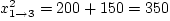 ; ; 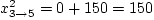 ; the rest of the remain zero. ; the rest of the remain zero.
Step 4:
Since , set k = 3 and select zone pair  as the next pair and go back to Step 3. as the next pair and go back to Step 3.
In this manner, Steps 3 and 4 are repeated till all the zone pairs are chosen (i.e., k = 16). Finally, the following assignment is obtained.
 = = |
450 |
|
 = = |
300 |
 = = |
650 |
 = = |
0 |
 = = |
0 |
 = = |
500 |
 = = |
450 |
 = = |
300 |
 = = |
650 |
 = = |
0 |
 = = |
550 |
 = = |
0 |
|