Capacity at facilities with uninterrupted traffic flow

Capacity is q_max and occurs at u = u₀  and k = k₀. Capacity analysis is that field of traffic engineering which tries to relate the design features of a transportation facility to the capacity it offers. In the case of facilities which offer uninterrupted traffic flow, like expressways, (or arterial sections with large inter-signal spacing), the design features are (i) the number of lanes, (ii) the width of lanes, (iii) the width of shoulders, and (iv) layout (like the frequency of curves and their curvatures, the general gradients, etc.). The purpose of capacity analysis is to see whether any of them affect capacity and if so what type of relation exists between them.

The question as to whether a design feature affects capacity is ultimately related to whether the design feature has any impact on the behaviour of drivers; i.e., whether the feature affects the speed-density relation (recall that speed-density relation is a product of driver behaviour). It has been observed, that all of the features mentioned above does have an impact on the speed-density relation and therefore on the capacity. Most of the time the reason for the impact is that drivers are affected psychologically by the presence or absence of a certain feature. For example, although, physically there is no reason why a narrower lane should impact driver behaviour yet the closeness of the edges affect a driver in such a way that a driver drives slower than usual.

For example, if the u-k relations on two roads with varying lane (road) widths are plotted then conceptually they may look something like what is shown in Figure 1. (The reason for using straight lines for the u-k relation is purely to make the figure easier to comprehend). As can be seen, chances are that both free flow speed and jam density will be lesser in the case of the narrow lane width road than in the case for a wide lane width road. Further, and more importantly, the speed at any given density is expected to be lower on the narrow road. This is because individual drivers will drive at a lesser speed at a given distance headway than they would have done on the wider road possibly due to a higher perception of threat to ones safety on the narrow road.

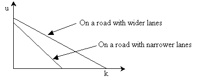
Figure 1: Conceptual u-k relations on lanes (roads) with different widths

Lower speeds at every density then would imply that flow at any density (or speed) will be lower for the narrower road and hence capacity will also be lower. The analysis of capacity concentrates on determining how the capacity value changes when any of the design features (like lane width) changes. In this sense, the scope of capacity analysis is narrow. However, recent trends show that traffic engineers are trying to determine the entire speed-density (or speed-flow) relationship with changing design features.

In the following, some observations on capacity of roads with different design features are listed:

1. Wider lanes increase capacity (per lane); however, beyond a certain value, the width of the lane stops playing any role in increasing capacity.
2. Wider shoulders increase capacity; like in the previous point, beyond a certain value the width of the shoulder does not affect capacity.
3. Straight, flat roads increase capacity; grades (or slopes in the vertical direction) affect capacity because it sometimes affect the performance of vehicles; horizontal curves always affect the way a driver drives because of the impact of the centrifugal acceleration and because of restricted sight distances.

In order to give the reader some idea of how these observations have been taken into account in working relations we discuss a method used by one of the most detailed capacity manuals, namely the Highway Capacity Manual (HCM) published by the Transportation Research Board of USA.

In the HCM method it is assumed that free speed (u_f ) of a stream on a given road indicates how drivers will behave over the entire range of density on that road. Hence being able to predict the free speed on a road with given specifications will allow one to determine the capacity of the road. This, in a nut-shell, is the basis on which capacity is determined by this method. Various tables and charts are presented which allow the engineer to determine what the free speed will be on a road with certain characteristics. Different speed-flow diagrams are provided and one needs to choose that which closely matches the free speed expected on the given road. This speed-flow diagram is then assumed to be the one for the given road. The capacity is simply read as the maximum flow as per the selected speed-flow diagram.

Other methods for determining capacity are also viable. For example, there are methods which define an ideal condition (in terms of road width, shoulder width, etc.) and a capacity value for this condition (often referred to as the ideal capacity ). Next these methods, define factors which reflect the proportion by which capacity has to be reduced for a given departure from the ideal condition. For example, if lane width is far removed from the ideal condition then one could define a proportion by which the capacity has to be reduced for such a departure. Typically, the product of all such reduction factors (from different parameters which are non-ideal) are determined and used as the factor by which the ideal capacity is reduced to reflect the capacity for non-ideal conditions.

Before leaving this discussion, it must be pointed out that the maximum number of vehicles that can cross a section (i.e. flow) obviously depends on the vehicle mix of the traffic stream. If the percentage of heavy vehicles (like trucks and buses) is more then it is expected that the total number of vehicles that cross a section will be lesser than in the case where all vehicles are, say, automobiles. Typically, the analysis of capacity is done assuming that all vehicles are automobiles. Hence when a stream contains different types of vehicles then the vehicles in the stream are converted to automobiles using an equivalency factor. For example, if a truck is considered to be equal to 2.5 automobiles then if a stream has 100 trucks per hour it is assumed that instead of trucks the stream has 250 automobiles per hour. The equivalency factors are referred to as passenger car (i.e., automobile) equivalency factors. Generally the passenger car equivalency factors for all types of vehicles are determined. These factors are used to convert a stream with a given mix of vehicles to an equivalent stream with only automobiles. The determination of equivalency factors is an issue which needs attention from researchers in the area and is beyond the scope of this lecture.