The cash flow diagram of Option-3 is shown here again for ready reference.

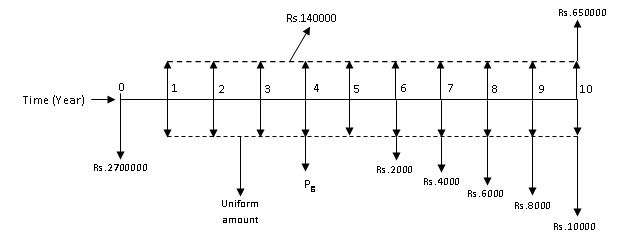
Fig. 2.10 Cash flow diagram of Option-3 with annual operating cost split into uniform base amount and gradient amount (shown for ready reference)

For the annual operating cost, the equivalent present worth of the gradient series starting from end of year ‘6' will be located at the end of year ‘4'. The future worth of this amount at end of year ‘10' will be determined by multiplying the equivalent present worth ‘ P_g ' (shown in Fig. 2.10) at the end of year ‘4' with the single payment compound amount factor (F/P, i, n) .

The equivalent future worth (in Rs.) of Option-3 is determined as follows;

Now replacing P_g with G (P/G, i, n) i.e. 2000( P/G, 8%, 6 ) in the above expression;

In the above expression, 2000 (P/G, 8%, 6) (F/P, 8%, 6) can also be replaced by 2000 (F/G, 8%, 6) .

Now putting the values of different compound interest factors in the above expression;

FW 3 = - Rs.3691336

Comparing the equivalent future worth of all the three alternatives, it is evident that Option-3 shows lowest negative equivalent future worth as compared to other options. Thus Option-3 will be selected for the purchase of the dump truck. This outcome obtained by future worth method is same as that obtained from the present worth method (Example-3) i.e. Option-3 is the most economical alternative.

After carrying out the comparison of equal life span mutually exclusive alternatives, now the illustration of future worth method for comparison of different life span mutually exclusive alternatives is presented.