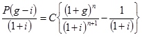
Subtracting equation (37) from equation (39) results in the following;

(40)

Equation (40) can be rewritten as follows;

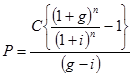(41)

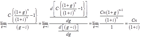
The expression in equation (41) is valid when g ≠ i. When ‘g' is equal to ‘i' then right hand side of the equation (41) takes the indeterminate form of . In this case the expression for the present worth ‘P' can be obtained by applying L'Hospital's rule as follows;

(42)

Then the expression for the present worth ‘P' is given as follows;

(43)

Similarly the future worth and equivalent uniform annual worth of the geometric gradient series can be obtained by multiplying its present worth ‘P' with the compound interest factors namely single payment compound amount factor (SPCAF) and capital recovery factor (CRF) respectively at the given rate of interest ‘i' per interest period and the number of interest periods.

Now using the above expressions, one can easily calculate the present worth, future worth and equivalent uniform annual worth of the cash flow involving either expenditure or income or both increasing in the form of geometric gradient.

It may be noted here that the expressions for compound interest factors can also be obtained by using beginning of year (interest period) convention.

The values of discrete compound interest factors at different values of interest rate and interest period can be calculated by using the expressions of these factors as mentioned earlier and the interest tables can thus be generated. The interest tables are available in the relevant texts (cited in the list of references for this course). The values of different discrete compound interest factors from these interest tables can directly be used in the engineering economy calculations.

The use of different compound interest factors discussed so far will be illustrated by solving various examples for comparison of different alternatives in Module 2. Further the use of discrete compound interest factors from interest tables will also be illustrated in Module 2.