First Approach: Invariance Approach
We can get the function W simply by substituting  in place of in place of  and using contracted notations for the strains in Equation (3.18). Noting that W is invariant, its form in Equation (3.18) must now be restricted to functional form and using contracted notations for the strains in Equation (3.18). Noting that W is invariant, its form in Equation (3.18) must now be restricted to functional form
 |
(3.25) |
From this it is easy to see that
Thus, the number of independent constants reduces to 9. The resulting stiffness matrix is given as
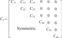 |
(3.26) |
When a material has (any) two orthogonal planes as planes of material symmetry then that material is known as Orthotropic Material. It is easy to see that when two orthogonal planes are planes of material symmetry, the third mutually orthogonal plane is also plane of material symmetry and Equation (3.26) holds true for this case also.
Note: Unidirectional fibrous composites are an example of orthotropic materials.
Second Approach: Stress Strain Equivalence Approach
The same reduction of number of elastic constants can be derived from the stress strain equivalence approach. From the first of Equation (3.12) and Equation (3.23) we have
 |
(3.27) |
The same can be seen from the stresses on a cube inside such a body with the coordinate systems shown in Figure 3.3. Figure 3.4 (a) shows the stresses on a cube with the coordinate system x1, x2, x3 and Figure 3.4 (b) shows stresses on the same cube with the coordinate system  . Comparing the stresses we get the relation as in Equation (3.27). . Comparing the stresses we get the relation as in Equation (3.27).
Now using the stiffness matrix given in Equation (3.20) and comparing the stress equivalence of Equation (3.27) we get the following:
This holds true when  . Similarly, . Similarly,
This gives us the  matrix as in Equation (3.26). matrix as in Equation (3.26).
|