
Next: Curve Fitting Up: Main Previous: Fixed point Iteration:
Bairstow Method
Bairstow Method is an iterative method used to find both the real
and complex roots of a polynomial. It is based on the idea of
synthetic division of the given polynomial by a quadratic function
and can be used to find all the roots of a polynomial. Given a
polynomial say,
 |
(B.1) |
Bairstow's method divides the polynomial by a quadratic function.
 |
(B.2) |
Now the quotient will be a polynomial

 |
(B.3) |
and the remainder is a linear function  , i.e.
 |
(B.4) |
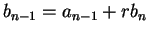
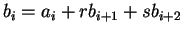
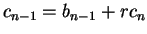
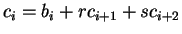
Since the quotient
 and the remainder are
obtained by standard synthetic division the co-efficients
and the remainder are
obtained by standard synthetic division the co-efficients
 can be obtained by the following recurrence relation.
 |
(B.5a) |
 |
(B.5b) |
 for for |
(B.5c) |
If

is an exact factor of

then the
remainder
is zero and the real/complex roots of
are the roots of
. It may be noted
that
is considered based on some guess values for

. So Bairstow's method reduces to determining the values of r
and s such that
is zero. For finding such values Bairstow's
method uses a strategy similar to Newton Raphson's method.
Since both

and

are functions of r and s we can
have Taylor series expansion of
,
as:
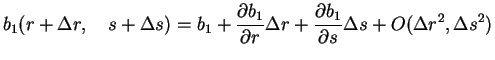 |
(B.6a) |
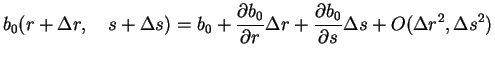 |
(B.6b) |
For
 ,
,
 terms
terms  i.e. second and higher order terms may be
neglected, so that
i.e. second and higher order terms may be
neglected, so that
 the improvement over
guess value
the improvement over
guess value  may be obtained by equating (B.6a),(B.6b) to
zero i.e.
may be obtained by equating (B.6a),(B.6b) to
zero i.e.
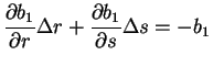 |
(B.7a) |
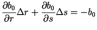 |
(B.7b) |
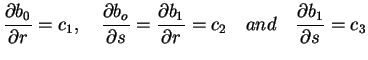
To solve the system of equations
, we need the
partial derivatives of

w.r.t. r and s. Bairstow has
shown that these partial derivatives can be obtained by synthetic
division of
, which amounts to using the recurrence
relation
replacing

with

and
with

i.e.
 |
(B.8a) |
 |
(B.8b) |
|
(B.8c) |
for 
where
 The system of equations (B.7a)-(B.7b) may be written
as.
The system of equations (B.7a)-(B.7b) may be written
as.
 |
(B.10a) |
 |
(B.10b) |
These equations can be solved for
and turn
be used to improve guess value to
 .
.
Now we can calculate the percentage of approximate errors in (r,s)
by
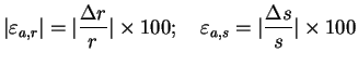 |
(B.11) |
If
 or
or
 , where
 is the iteration
stopping error, then we repeat the process with the new guess
i.e.
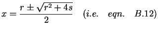
. Otherwise the roots of
can be determined by
is the iteration
stopping error, then we repeat the process with the new guess
i.e.
. Otherwise the roots of
can be determined by
 |
(B.12) |
If we want to find all the roots of then at this point
we have the following three possibilities:
-
If the quotient polynomial
is a third (or higher)
order polynomial then we can again apply the Bairstow's method to
the quotient polynomial. The previous values of
can serve
as the starting guesses for this application.
- If the quotient polynomial
is a quadratic
function then use (B.12) to obtain the remaining two roots of
.
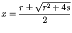
- If the quotient polynomial
is a linear function
say
 then the remaining single root is given by
Example:
Find all the roots of the polynomial
by Bairstow method . With the initial values
Solution:
Set iteration=1
Using the recurrence relations (B.5a)-(B.5c) and
(B.8a)-(B.8c) we get
 the simultaneous equations for
  and
and  are:
on solving we get
are:
on solving we get
and
Set iteration=2
Now on using
we get
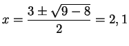
So at this point Quotient is a quadratic equation
Roots of  are:
are:
 Roots
Roots  are
are
i.e

Exercises:
(1) Use initial approximation  to find a quadratic factor of the form
  of the polynomial equation
using Bairstow method and hence find all its roots.
(2) Use initial approximaton  to find a quadratic factor of the form of the polynomial equation
using Bairstow method and hence find all the roots.
Next: Curve Fitting Up: Main
Previous: Fixed point iteration: