In this section, we will look at some special classes of square
matrices which are diagonalisable. We will also be dealing with
matrices having complex entries and hence for a matrix
![$ A=[a_{ij}],$](img31.png) recall the following definitions.
recall the following definitions.
Note that a symmetric matrix is always Hermitian, a skew-symmetric matrix
is always skew-Hermitian and an orthogonal matrix is always
unitary. Each of these matrices are normal. If  is a unitary
matrix then
is a unitary
matrix then

EXAMPLE 6.3.2
- Let
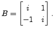 Then
Then  is skew-Hermitian.
- Let
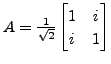 and
and
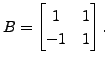 Then
is a unitary matrix and
is a normal
matrix. Note that
Then
is a unitary matrix and
is a normal
matrix. Note that
 is also a normal matrix.
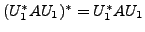
EXERCISE 6.3.4
- Let
be a square matrix such that
 is a diagonal matrix for some unitary matrix
  .
Prove that
is a normal matrix.
.
Prove that
is a normal matrix.
- Let
be any matrix. Then
 where
where
 is the Hermitian part of
and
is the Hermitian part of
and
 is the skew-Hermitian part of
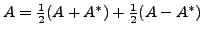
- Every matrix can be uniquely expressed as
 where both
  and
and  are Hermitian matrices.
- Show that
 is always skew-Hermitian.
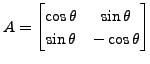
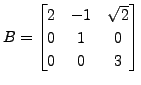
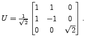
- Does there exist a unitary matrix
such that
 where
where
 and
and
Proof.
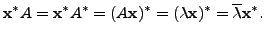
Let

be an eigenpair. Then

and

implies
Hence
But

is an eigenvector and hence

and so the real number

is non-zero as well. Thus

That is,

is a real number.
height6pt width 6pt depth 0pt
Proof.
We will prove the result by induction on the size of
the matrix. The result is clearly true if

Let the result
be true for

we will prove the result in case

So, let
be a

matrix and let

be
an eigenpair of
with

We now extend the linearly
independent set

to form an orthonormal basis
(using
Gram-Schmidt
Orthogonalisation) of

.
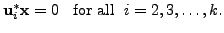
As
is an orthonormal set,
Therefore, observe that for all

Hence, we also have

for

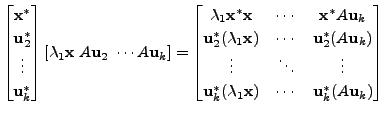
Now, define
![$ U_1 = [ {\mathbf x}, \; {\mathbf u}_2, \; \cdots, {\mathbf u}_k ]$](img3023.png)
(with

as columns of

). Then the matrix
is a unitary matrix
and
where
is a
matrix. As

,we get
. This condition,
together with the fact that

is a real number (use Proposition
6.3.5), implies that

. That is,
is also
a Hermitian matrix. Therefore, by induction hypothesis there
exists a
unitary matrix

such that
Recall that , the entries

for

are the eigenvalues of the matrix

We also know that
two similar matrices have the same set of eigenvalues. Hence, the
eigenvalues of
are
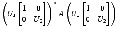
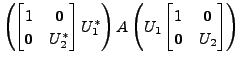
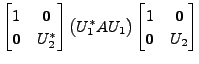
Define
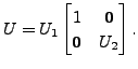
Then
is a unitary matrix
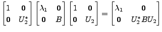
and
Thus,

is a diagonal matrix with diagonal entries
the eigenvalues of
Hence, the result follows.
height6pt width 6pt depth 0pt
COROLLARY 6.3.7
Let
be an
 real symmetric matrix. Then
- the eigenvalues of
are all real,
- the corresponding eigenvectors can be chosen to have real entries, and
- the eigenvectors also form an orthonormal basis of

Proof.
As
is symmetric,
is also an Hermitian matrix. Hence, by Proposition
6.3.5, the eigenvalues of
are all real.
Let

be an eigenpair of
Suppose

Then there exist

such that

So,
Comparing the real and imaginary parts, we get

and

Thus, we can choose the eigenvectors to have real entries.
To prove the orthonormality of the eigenvectors, we proceed on the lines
of the proof of Theorem 6.3.6, Hence, the readers are advised
to complete the proof.
height6pt width 6pt depth 0pt
Remark 6.3.9
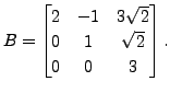
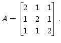
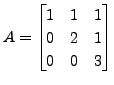
In the previous exercise, we saw that the matrices
 and
and
 are similar but not unitarily equivalent, whereas
unitary equivalence implies similarity equivalence as
are similar but not unitarily equivalent, whereas
unitary equivalence implies similarity equivalence as
 But in numerical calculations, unitary transformations are preferred
as compared to similarity transformations. The main reasons being:
But in numerical calculations, unitary transformations are preferred
as compared to similarity transformations. The main reasons being:
- Exercise 6.3.8.2 implies
that an orthonormal
change of basis leaves unchanged the sum of squares of the
absolute values of the entries which need not be true under a
non-orthonormal change of basis.
- As
 for a unitary matrix
  unitary equivalence is
computationally simpler.
unitary equivalence is
computationally simpler.
- Also in doing ``conjugate transpose", the loss of accuracy due to round-off
errors doesn't occur.
We next prove the Schur's Lemma and use it to show that normal matrices
are unitarily diagonalisable.
LEMMA 6.3.10 (Schur's Lemma)
Every
complex matrix is unitarily similar to an upper
triangular matrix.
Proof.
We will prove the result by induction on the size of
the matrix. The result is clearly true if
Let the result
be true for
we will prove the result in case
So, let
be a
matrix and let
be
an eigenpair for
with
Then the linearly
independent set
can be extended, using the
Gram-Schmidt
Orthogonalisation process, to get an orthonormal basis
of

. Then
![$ U_1 = [ {\mathbf x}\; {\mathbf u}_2 \; \cdots {\mathbf u}_k ]$](img3081.png)
(with
as the columns of the matrix
)
is a unitary matrix and
where
is a
matrix. By induction
hypothesis there exists a
unitary matrix
such that

is an upper triangular matrix
with diagonal entries

the eigen
values of the matrix
Observe that since the eigenvalues of
are

the
eigenvalues of
are
Define
Then check that
is a unitary matrix and
is an upper triangular matrix with diagonal entries
the eigenvalues of the
matrix
Hence, the result follows.
height6pt width 6pt depth 0pt
We end this chapter with an application of the theory of diagonalisation
to the study of conic sections in analytic geometry and the study of
maxima and minima in analysis.
A K Lal
2007-09-12


![$\displaystyle \left[\begin{array}{c\vert c} \lambda_1 & {\mathbf 0}\\ \hline {\mathbf 0}& \\
\vdots & B \\ {\mathbf 0}& \end{array} \right],$](img3029.png)


 corresponding to distinct eigenvalues
 satisfy
 is
an eigenpair for
is
an eigenpair for 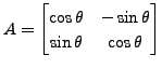 for some

 for some
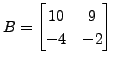
 Determine
  is a two dimensional rotation of

![$\displaystyle \begin{bmatrix}{\mathbf x}^* \\ {\mathbf u}_2^* \\ \vdots \\ {\ma...
..._1 & * \\ \hline {\mathbf 0}& \\ \vdots & B \\ {\mathbf 0}&
\end{array} \right]$](img3082.png)
 and
and
 are unitarily equivalent via the unitary matrix
 Hence, conclude that
the upper triangular matrix obtained in the "Schur's Lemma" need
not be unique.
Hence, conclude that
the upper triangular matrix obtained in the "Schur's Lemma" need
not be unique.