Most of the Circuit elements have at least two leads (electrical terminals). They are characterized by voltage across the terminals and current flowing through the device (see Fig.2.1); this is V-I characterization of device.
Resistance: Across this element, if we applied a voltage source
and observe the current, then we will observer that
![]() , that
is,
, that
is, ![]() , where R is the resistance measured in Ohms
(Fig.1.1, 2.2).
, where R is the resistance measured in Ohms
(Fig.1.1, 2.2).
Higher the value of R, larger the voltage required to achieve the same current. Voltage proportional to current - is Ohm's law (It was deduced hueristically by experiments for metals, by George Simon Ohm). For lamp, this law is not true, as with increase in current, temperature of bulb increases, causing the increase in resistance. Hence Ohms law is not strictly true for lamp. But for most of the practical purposes and for this course the Ohm's law holds true for the resistive circuit elements.
The resistive elements (resistances) can be fixed or variable. Commonly use resistor types are carbon film and wirewound. The example of variable resistor is potentiometer.
For a material with length ![]() and cross-sectional area
and cross-sectional area ![]() , the
resistance will be
, the
resistance will be
![]() , where
, where ![]() is specific
resistivity (property of material). Inverse of resistance is
conductance.
is specific
resistivity (property of material). Inverse of resistance is
conductance.
![]() , measured in mhos or Seimens.
, measured in mhos or Seimens.
In Fig. 2.4, property of interest is resistance between A and B. It is dependent on details of wire, connector, filament, material, and shape. It can be abstracted as simple resistance (Fig.2.4).
Inductance:
It another important basic circuit element.
Current flowing in a wire causes generation of magnetic field intensity
(
![]() ).
).
![]() is independent of material medium surrounding the current
carrying wire. The
is independent of material medium surrounding the current
carrying wire. The
![]() leads to magnetic flux density
leads to magnetic flux density
![]() .
Here
.
Here ![]() is absolute permeability of vaccum.
is absolute permeability of vaccum. ![]() is relative
permeability of material where
is relative
permeability of material where ![]() is measured. The flux flowing around
wire links with the conducting wire. And if the flux linkage changes it
lead to generation of EMF (electromotive force) which try to oppose the
change in flux. This means it tries to nullify the change in current.
is measured. The flux flowing around
wire links with the conducting wire. And if the flux linkage changes it
lead to generation of EMF (electromotive force) which try to oppose the
change in flux. This means it tries to nullify the change in current.
The current ![]() causes production of magnetic flux.
causes production of magnetic flux.
![]() is the EMF of a single turn. Here,
is the EMF of a single turn. Here, ![]() .
Thus, the total EMF
.
Thus, the total EMF
![]() , where
, where ![]() is the number of turns.
is the number of turns.
Defining the inductance -
![]() ,
, ![]() is inductance and measured in Henry.
See the output current of sinusoidal
is inductance and measured in Henry.
See the output current of sinusoidal ![]() applied across an inductor in
Fig.2.5
applied across an inductor in
Fig.2.5
In lumped model, inductance is considered only due to element. The inductance due to wires connecting it to other elements is neglected (Fig.2.6)
Analysis of circuit: To find voltage or currents in an element of interest. One can also find voltage and current in all the elements of circuit.
Lumped simplified model of resitance, inductance and capacitance.
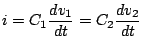
Capacitance:
![]() ,
, ![]() capacitance.
The magnitude of charge on either plate is given by
capacitance.
The magnitude of charge on either plate is given by ![]() .
.
Lumped model: Shape, material, wire, connectors - effect of each is assumed to be due to single entity shown by the symbols in the diagram. In actual resistance, inductance and capacitance are distributed all across the circuits. For most practical purpose, lumped model- satisfactory.
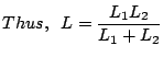
Series and Parallel connections
Kirchoff's volatage law: In a circuit, if your start from a point A and tranverses the circuit in any fashion and reaches back to point A, the total sum of potential changes should be zero. This has to be true since, same point cannot have two different potentials.
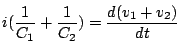
Kirchoff's current law: At any point in the network, total amount of current entering and leaving the point has to be equal to rate of accumulation of charge at the point. Since, in the circuits ordinarily the points where one circuit element is connected to other circuit element (these points are called nodes) do not store charge sum of incomming current has to be equal to sum of outgoing currents.
Thus, for series model, we get relations:
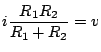
For parallel connection, we get the relations:
 |
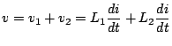
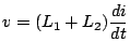
Inductances in series:
 |
|||
 |
|||
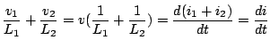
Inductances in parallel:
 |
|||
 |
|||
 |
|||
 |
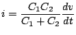
Capacitances in series:
 |
|||
 |
|||
 |
|||
 |
Capacitances in parallel
 |
|||
|
|||
 |
|||
Inductance of a Solenoid (Coil)
Define ![]() =magnetic circuit path length
=magnetic circuit path length
A=magnetic circuit crossectional area.
Inductance: (Assuming that ![]() is same in the closed path of
length
is same in the closed path of
length ![]() .)
.)
 |
|||
 |
|||
 |
|||
 |
|||
 |
|||
 |
|||
 |
Here
![]() is magnetomotive force (equivalent of eletromotive
force - EMF in magnetic domain), and flux
is magnetomotive force (equivalent of eletromotive
force - EMF in magnetic domain), and flux ![]() is equivalent of
current in magnetic domain. The Magnetic reluctance=
is equivalent of
current in magnetic domain. The Magnetic reluctance=
![]() is
then equivalent of resistance in magentic domain.
is
then equivalent of resistance in magentic domain.
Linearity: when elemental change in cause ![]() , always
leads to same elemental change in effect i.e.,
, always
leads to same elemental change in effect i.e., ![]() , then the
system is said to be linear.
, then the
system is said to be linear.
In general, for a system let input ![]() lead to output
lead to output ![]() , and a
small perturbation in
, and a
small perturbation in
![]() causes a small perturbation
causes a small perturbation
![]() in output. If perturbation
in output. If perturbation
![]() alwasy leads to same
perturbation of
alwasy leads to same
perturbation of
![]() in the output irrespective of any
in the output irrespective of any ![]() ,
then the system is linear.
,
then the system is linear.
The implication of the above is that if input ![]() causes output
causes output
![]() , and
, and ![]() causes
causes ![]() , then
, then
![]() will
cause an output of
will
cause an output of
![]() . This is principal of
superposition.
. This is principal of
superposition.
![\includegraphics[width=3.0in]{lec1figs/fig1.eps}](img16.png)
![\includegraphics[width=3.0in]{lec1figs/fig3.eps}](img19.png)
![\includegraphics[width=3.0in]{lec1figs/fig4.eps}](img25.png)
![\includegraphics[width=3.0in]{lec1figs/fig5.eps}](img26.png)
![\includegraphics[width=3.0in]{lec1figs/fig8.eps}](img39.png)
![\includegraphics[width=3.0in]{lec1figs/fig9.eps}](img40.png)
![\includegraphics[width=3.0in]{mainfigs/symbols.eps}](img44.png)
![\includegraphics[width=3.0in]{lec1figs/fig12.eps}](img45.png)
![\includegraphics[width=3.0in]{lec1figs/fig16.eps}](img62.png)
![\includegraphics[width=3.0in]{lec1figs/fig18.eps}](img70.png)