8.2.1 Simple Hypothesis Testing
In detection theory, a hypothesis is a statement about the source of the observed data. In the simplest case, we have the null hypothesis ( 0) that there is no change from the usual and the alternate hypothesis (1) that there is a change. For example. in the target detection problem, the hypotheses may be
![H0 : x[0 ] = w [n] H1 : x[0 ] = 1 + w [n ]](images/1.jpg)
and the objective is to decide which one of these hypothesis is true based on the observed data.
We begin with those decision making problems in which the PDF for each assumed hypothesis is completely known, that is why they are referred to as simple hypothesis testing problems. The primary approaches to simple hypothesis testing are the classical approach based on Neyman-Pearson theorem and the Bayesian approach based on minimization of the Bayes risk. In many ways these approaches are analogous to the classical and Bayesian methods of statistical estimation theory.
8.2.2 Neyman-Pearson (NP) Detector
Before explaining the NP detector, we first describe some relevant terminologies. Suppose we observe realization of a random variable whose PDF is either  (0, 1) and (1, 1). The detection problem cam be summarized as:
![( ) ---1--- -1-- 2 p(x[0 ];H0 ) = √ ----2 exp 2σ2 x [0] 2π σ ( ) p(x[0 ];H ) = √--1---exp -1--(x[0] - 1)2 1 2π σ2 2σ2](images/3.jpg)
where 0 is referred to as the null hypothesis and 1 as the alternate hypothesis.
The PDFs under each hypothesis along with the probabilities of hypothesis testing errors as shown in Figure 8.1. A reasonable approach might be to decide 1 if x[0] > 1∕2. This is because if x[0] > 1∕2 the observed sample more likely if 1 is true. Our detector then compares the observed datum value with 1∕2, which is called threshold.
With this scheme we can make two errors. If we decide 1 but 0 is true, we make Type I error. On the other hand, if we decide 0 when 1 is true, we make a Type II error. The terms Type I and Type II errors are use in statistical domain but in engineering domain these errors are referred to as false alarm and miss, respectively. The term P(i; j) indicates the probability of deciding i when j is true. Note that it is not possible to reduce both error probabilities simultaneously. A typical approach is to hold one error probability value fixed while minimizing the other.
![1 ( 1 ) p(x[0];A) = √-----2 exp - ---2(x[0] - A )2 2π σ 2σ](images/5.jpg)
Figure 8.1: PFDs in binary hypothesis testing, possible errors and their probabilities
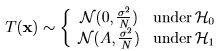
In general terms the goal of a detector is to decide either 0 or 1 based on observed data
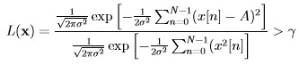
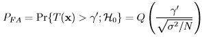
x = [x[0] x[1]… x[N - 1]]T. This is a mapping from each possible data set value into a decision. The decision regions for the previous example are shown in Figure 8.2. Let R1 be the set of values in RN that map into decision 1. Then probability of false alarm PFA (i.e., Type I error) is computed as:
![p(x[0 ];H0 ) : A = 0 p(x[0 ];H1 ) : A = 1](images/6.jpg)
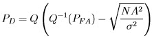
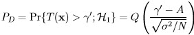
where α is termed as significance level or size of the test in statistics. Now there are many R1 that satisfy the above relation. Our goal is to choose the one that maximizes the probability of detection defined as:
![( ) 1 1 2 p(x[0]|H0 ) = √-----2 exp - --2x [0] 2πσ ( 2σ ) ---1--- -1-- 2 p(x[0]|H1 ) = √2-πσ2-exp - 2σ2(x [0] - 1)](images/7.jpg)
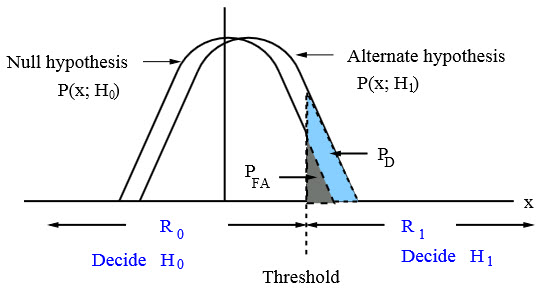
Figure 8.2: Decision regions in binary hypothesis testing
Neyman-Pearson Theorem: To maximize the PD for a given PFA = α decide 1 if:
![]()
where the threshold γ is computed from the constraint on the probability of false alarm value:
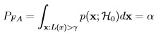
Then function L(x) is termed the likelihood ratio and the entire test is called as likelihood ratio test (LRT).
![[ ] ⌊ x[0]⌋ ˆ T - 1 T x [0 ] ˆ ⌈ ⌉ θ = (H H ) H x = x [1 ] and ˆs = H θ = x[1] 0](images/13.jpg)
 .
.