4.3.1 MLE for Transformed Parameters
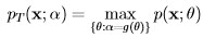
The MLE of the transformed parameter, α = g(θ) is given by:

where  is the MLE of θ. If g is not one-to-one function (i.e., not invertible) then
  is obtained as the MLE of transformed likelihood function, pT (x; α), which is defined as:
4.3.2 Example
In this example we demonstrate the finding of transformed MLE. In context of the previous example, consider two different parameter transformations (i) α = exp(A) and (ii) α = A².
Case (i) From previous example, the PDF parameterized by the parameter θ = A can be given as
![[ N∑ -1 ] p(x;A ) = ----1--N-exp - -1-- (x[n ] - A )2 - ∞ < A < ∞ (2πσ2 )2- 2σ2 n=0](images/3.jpg)
Since α is a one-to-one transformation of A, the PDF parameterized in terms of the transformed parameter can be given as
![[ ] 1 1 N∑ -1 pT(x; α) = -------N-exp - ---- (x[n ] - lnα )2 α > 0 (2π σ2)2 2σ2 n=0](images/4.jpg)
Thus pT (x; α) is the PDF of the data set,
![x [n ] = ln α + w[n] n = 0,1,...,N - 1](images/5.jpg)
Now to find the MLE of α, setting the derivative of pT (x; α) with respect to α to zero yields
![N∑- 1 1 (x[n] - ln ˆα )--= 0 n=0 ˆα](images/6.jpg)
or

But  being the MLE of A, so we have = exp(Â). Thus the MLE of the transformed parameter is found by substituting the MLE of the original parameter into the transformation function. This is known as invariance property of MLE.
Case (ii) Since  , the α is not one-to-one transformation of A. If we take
  only then some possible PDFs will be missing. To characterize all possible PDFs, we need to consider two sets of PDFs
![[ N∑- 1 -- ] pT1(x;α) = ----1----exp - -1-- (x [n ] - √ α)2 α ≥ 0 (2πσ2 )N2- 2σ2 n=0 [ N- 1 ] ----1---- -1--∑ √ --2 pT2(x;α) = 2 N2-exp - 2σ2 (x [n ] + α) α > 0 (2πσ ) n=0](images/11.jpg)
The MLE of α is the value of α that yields the maximum of pT1(x; α) and pT2(x; α) or
![αˆ = argmaxα [pT1(x;α),pT 2(x; α)]](images/12.jpg)
The maximum can be found in two steps as
- For a given value of α, say α0, determine whether pT1(x; α) or pT2(x; α) is larger. If for example pT1(x; α0) > pT2(x; α0) then denote the value of pT1(x; α0) as
 . Repeat for all α > 0 to form
  . Note that
 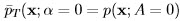 .
.
- The MLE is given as the α that maximizes over α ≥ 0.
Thus the MLE is
![√ -- √ -- ˆα = arg max [pT1(x; α ),pT 2(x; - α)] [ α ] √ -- √ -- 2 = arg m√ax {pT 1(x; α),pT2(x;- α )} [ α≥0 ] 2 = arg -∞ma<xA<∞ p (x; A) = Aˆ2 = ¯x2](images/16.jpg)
Again the invariance property holds.
4.3.3 MLE for General Linear Model
Consider the general linear model of the form:
x = Hθ + w
where H is a known N × p matrix, x is an N × 1 observation vector with N samples, and w is N × 1 noise vector with PDF  (0,C). The PDF of the observed data is:
![1 [ 1 ] p(x;θ) = ----N----1----exp - -(x - H θ)TC -1(x - H θ) (2 π)2 det2(C ) 2](images/17.jpg)
and the MLE of θ is found by differentiating the log-likelihood which can be shown to yield:
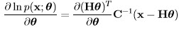
which upon simplification and setting to zero becomes:
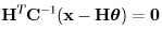
and this yields the MLE of θ as:
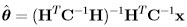
which turns out to be same as the MVU estimator.