(a) Consider the signal shown below.

Fig. (a)

Now consider convolution of with itself. Let the resultant signal be .

Then, .

Now, consider and .

Fig (b)

Fig (c)

So, when .

as there is no overlap between and .

When .

Then, .

Here, and .

So, .

               .

When .

Then, there is no overlap between and .

So, the signal is

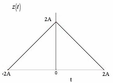
Fig. (d)

 Now compare with the given signal . Here is

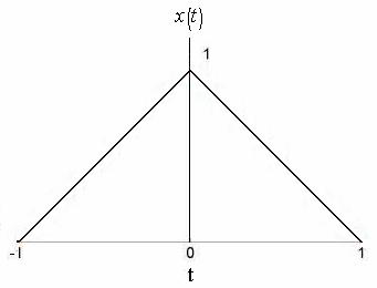
Fig. (e)

By comparing, we get .

So, can be thought of as a signal which is a convolution of the signal with itself, where is

Fig. (f)

This implies .

By Convolution Theorem, the Fourier Transform of is square of the Fourier Transform of , i.e. .

Now, consider . Its Fourier Transform is

            .

So,

.

(b)

Now, consider a signal , where

as .

So, is the shifted version of by 4k along the t axis which is shown as

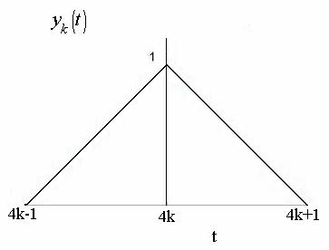
Fig. (g)

Now,

So, is

Fig. (h)

(c) Any signal which is the shifted version of by 4k on the t axis can be taken as , which satisfies because by the last part we can say that when we convolve with , it will result in .

In this case, , where .

(d) By part (c) ,

, where .

.

Now, put .

as