| Fundamental concepts of semiconductors |
| |
| |
| |
| |
| |
| 1.3 Dynamics of electrons in periodic potential |
| |
In order to see how an electron(s) behaves in a crystalline environment,
we treat the electrons in a simple periodic potential, which is, for some extent, is a useful approximation.
|
From your modern physics background you are aware that, each atom contains several electrons
and they occupy a specific state. In such cases, Schrödinger equation effectively explains the probability of
finding an
electron, and also
one can easily extend it to many electron systems. Let us take an example: Isolated carbon atoms contain 6 electrons, which occupy
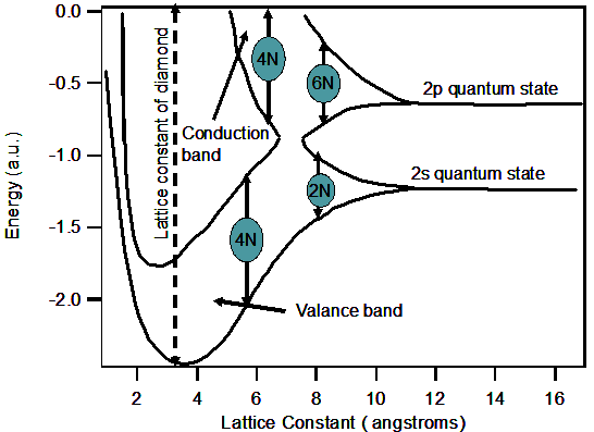
the 1s, 2s and 2p orbital in pairs. Energies of an electron occupying the 2s and 2p orbital are indicated in the figure 2.11. As the
lattice constant is reduced, there is an overlap of the electron wave functions occupying adjacent atoms. This leads to the splitting
of the energy levels, which is consistent with the Paulis exclusion principle. The splitting results in an energy band containing 2N
states in the 2s band and 6N states in the 2p band, where N is the number of atoms in the crystal. A further reduction causes the 2s and 2p
energy bands to merge and split again into two bands containing 4N states each.
|
| |
|
Fig.2.11 Schematic representation of energy band development for Diamond upon reduction in the lattice constant .
Here we see the splitting of energy into a band of allowed and forbidden energy levels.
|
| |
Now the lower band is completely filled with electrons at zero temperature,
which is
labeled as the valence band. The upper band, which is empty, is the conduction band. We can also use the example of Si.
Each atom of Si has 14 energy levels, corresponding to 14 electrons. Now there are 1022 atoms in a cubic centimeter.
Now imagine the complexity of the energy levels!! There are some regions where electron propagation is completely forbidden,
and such gap is called as forbidden gap.
|
| |
We can still go further to explain this band formation, by using periodic potential
functions known as Bloch functions. Here we have to consider a detailed quantum mechanical treatment, on which band
theory is based on. However, we will try to minimize the rigorous mathematical treatment wherever it is possible.
The theory we are about to discuss, generalizes the electron propagation in a crystal assuming electron states are
Bloch states. As you might have studied in previous classes, electrons propagating in plane-wave states, corresponding
to free electrons, are having sharp momentum  , where k is the momentum vector. As we are considering crystal periodicity
as ionic potential, electron function is also periodic. That is electrons states are now periodic Bloch states, , where k is the momentum vector. As we are considering crystal periodicity
as ionic potential, electron function is also periodic. That is electrons states are now periodic Bloch states,
|
|
The Bloch states satisfy the Schrödinger equation for a periodic potential V(r) which could be written as
|
|
To understand the influence of the periodic potential on electron motion in a crytstal,
we first determine the velocity and correlate it to the energy of the electron.
The instantaneous velocity of electron in the quantum mechanical treatment of moving electron is
|
|
After solving Schrödinger equation, we get(generalizing to three dimensional)
 . That means the velocity is simply proportional to the gradient
of energy as a function of momentum vector k. If we look at the rate of change of velocity, by taking time derivative,
we obtain . That means the velocity is simply proportional to the gradient
of energy as a function of momentum vector k. If we look at the rate of change of velocity, by taking time derivative,
we obtain  , which is quite analogous to the Newtons second law, relating
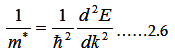
left-hand side to the acceleration and the right side of the ratio of the force to the mass. Here the effective mass
of electron demonstrates the energy dependence, suggesting that the fact that the electron mass is different at various
energy levels. Here we can extract effective mass expression, as , which is quite analogous to the Newtons second law, relating
left-hand side to the acceleration and the right side of the ratio of the force to the mass. Here the effective mass
of electron demonstrates the energy dependence, suggesting that the fact that the electron mass is different at various
energy levels. Here we can extract effective mass expression, as
|
|
One can also obtain the effective mass in different ways. In other words, the motion of
electrons in a crystal could be treated identically as a free particle, but with the effective mass replacing free electron mass.
Use of effective mass in our subsequent sections is enormous; we often represent many expressions with respect to effective
mass. However, the applicability of the expression (2) is not always valid, as we derived it only at the band edge.
In later sections, we see how m* vary at different energy levels and thus other parameters.
As we have seen now the free electron model, where the energy (E)-momentum (k)
relation
is in simple parabolic, can not explain the
energy gap. In the following section we shall see how certain discrete energies are allowed and some or not.
|
| |
| |
| |
| |
| |
| 1.3.1 Kronig-Penny Model |
| |
Here we are going to show that in any periodic potential, only certain
discrete energies are allowed and such allowed energies form a band. We also show how a gap of energies
that are forbidden, wherein no electron propagation would occur.
|
|
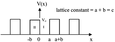
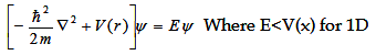
Fig.2.12 . One dimensional periodic potential with height Vo and the width is b.
Note that the lattice constant is a+b, where a is the gap between potentials.
|
| |
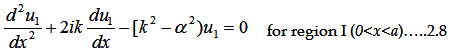
Let us examine the solution of the Schrödinger equation for an arbitrary periodic potential (V(x)).
For mathematical convenience, we restrict ourselves to only one dimension, with the assumption that it is subsequently
true for the real 3D systems. Another assumption is using a regular periodic potential (with a lattice constant of a+b,
as shown in figure 2.12).
The Schrödinger equation is
|
|
For 1D the whole equation turns to
|
|
Where V(x) is periodic and hence it must satisfy V(x)=V(x+(a+b)).
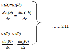
If you look closely the figure 2.12, there are two regions, -b < x < 0 and 0 < x < a, where the potential is
zero and V0 in respective regions.
As both these regions are solvable in the Bloch function, considering the potential
being
periodic and the wave
function Ψk (X) = unk(X)eikx is also periodic.
|
Hence for Eq.2.7 will get two solutions for both the regions and
then we
have to apply
boundary conditions at x=0 and x=a (it also same for x=-b)
The simplified equation 2.7, after substituting the wave function, we get
|
|
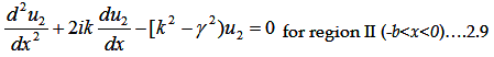
|
|
Corresponding solutions for region I and II are
|

|
The coefficients A, B, C and D can be only determined by applying boundary conditions.
Now, since the barrier is finite, there must be some probability of penetration by the electrons. Therefore,
both the wave function and its first derivative must be continuous at points such as x = 0, x=a and also at x=-b.
This allows us to establish relationships between the constants A, B, C and D.
That means
|
|
Substituting the wave functions in above boundary condition results into four sets of equations,
containing A, B, C and D coefficients (try
yourself!
).
Excluding very trivial solutions, these
equations
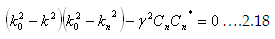
have only a single solution if the determinant of the coefficients of A, B, C and D vanishes if,
|

|
The above condition is valid only when the energy of the electron is greater than the
potential energy (E>V0 ). When the energy is less than the potential energy then ϒ will be imaginary. One can
transform the imaginary arguments in terms of hyperbolic functions as
|
Sin ix=isinh(x), cosix =cosh(x)
|
Therefore the above expression changes to
|

|
Now consider a condition b→ 0 and V0 → infinity (This would not disturb any of our primary
conditions). Then equation turns to
|
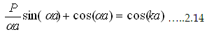
|
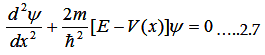
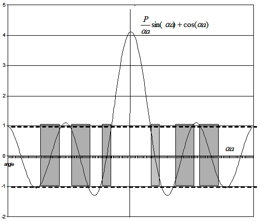
Where  . This we can solve graphically for P=3π/2. The first term is plotted
in figure2.13 as a function of αa . This figure suggests that the 1st term allows only certain values as the
second term is between +1 and -1. Because αa is a function energy, the limitation means electrons in a periodic
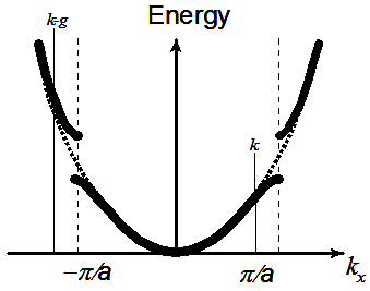
potential can occupy only certain levels. Similarly, we can justify easily the case for E>V0. Fig2.14 gives the Energy
dispersion for a particle in a periodic potential (dashed line is a representative for free particle dispersion). Note
that the presence of gap is in multiples of π/(a+b), that corresponding to imaginary part of k vector. . This we can solve graphically for P=3π/2. The first term is plotted
in figure2.13 as a function of αa . This figure suggests that the 1st term allows only certain values as the
second term is between +1 and -1. Because αa is a function energy, the limitation means electrons in a periodic
potential can occupy only certain levels. Similarly, we can justify easily the case for E>V0. Fig2.14 gives the Energy
dispersion for a particle in a periodic potential (dashed line is a representative for free particle dispersion). Note
that the presence of gap is in multiples of π/(a+b), that corresponding to imaginary part of k vector.
|
|
Fig.2.13 A plot of 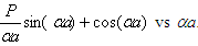 . Shaded region is the allowed values corresponding to real k. . Shaded region is the allowed values corresponding to real k.
|
Thus, we can write the following conclusions from the above:
|
- All real- k vectors lead to propagate electron states in a crystal. Consequently, these states have allowed states
- On the other hand, the energies corresponding to the imaginary k vectors cannot propagate in the crystal, therefore the forbidden gap.
- If the potential barrier between the walls is strong, energy bands are narrow and wide apart.
- If the potential barrier is weak, energy bands are wide and closely packed. (This is a typical condition of metals with weakly bond electrons. Here nearly- free electron model works well)
|
|
Fig.2.14 Schematic extended zone model. Dashed line representative of free electron model
|
| |
| |
| |
| 1.3.2 Nearly- free electron model |
| |
Let us discuss another classic model for an electrons in a periodic potential. Previously,
we examined how an electron behaves in rectangular periodic potential. We have witnessed that such system will lead to a
set of allowed and forbidden energies of electron. But still we are not sure, how such methodology could be applied for
any arbitrary potential.
Once again, we have to use Schrödingers equation and here the potential is arbitrary, but still maintaining its periodicity
with lattice constant, a.
So we can write the potential as a function of x as
|
|
Wherein The function 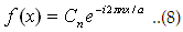 (You can also express Cn in term of f(x)) (You can also express Cn in term of f(x))
|
The electronic functions ( Bloch functions) must also maintain the same
periodicity as well, that is Ψnk(r) = unk(X)eikr .
|
If an electron is completely free then V(x) as well as γ are zeros. However,
in a week potential, γ may have a reasonably good value. Hence the Bloch function could be re-written as 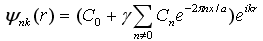 .
This equation is a combination of a simple plane wave and a periodic part contribution. .
This equation is a combination of a simple plane wave and a periodic part contribution.
|
We can solve the Schrödinger equation by defining the following, without any
compromise, k=kn+2Πn/a and k=km+2Πm/a within the periodicity.
Let us also use the orthogonality of plane wave:
|
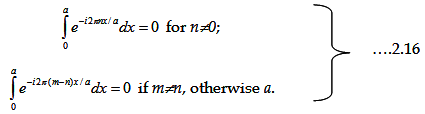
|
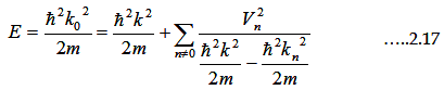
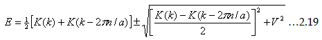
After several mathematical manipulations we ultimately get the expression for the Energy
|
|
where 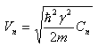
|
Equation 2.17
consists
of both free-electron component as well as small correction term.
Let us examine further and see what happens at the Brillouin zone boundaries, ie., k=nΠ/a. As you observe, the second
term vanishes if k2=kn2. That means the energy as well as wave function diverges at that situation. As a result of that,
γ and Cn are no longer small.
Use the Wave function as given previously and reduce the coefficients into
|
|
| Finally the energy is determined as
|
|
(remember  similarly others) similarly others)
|
At zone edge (k=kn=nΠ/a), The above relation simply gives us 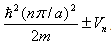 which shows a clear gap of E(k) relating the first Brillouin zone, to the magnitude equal to 2Vn. which shows a clear gap of E(k) relating the first Brillouin zone, to the magnitude equal to 2Vn.
|
More precisely, any two states which are scattered into each other by a potential
V will produce new states which are now a mixture of the original ones E1 and E2 and with
new energies.
|
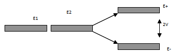
Fig 2.15 Schematic of energy split
|
These new states are centered around the average energy of the original two states,
but are split apart by an amount which is the mean square average of their initial separation and the strength of the
scattering. Schematically it is represented in fig 2.15
|
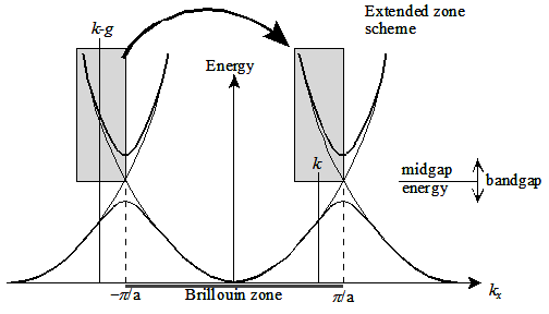
|
Fig.2.16 (a) Dispersion relation for nearly-free electrons (thick) and free electrons
(b) Dispersion relation for nearly-free electrons in the extended zone scheme
|
| |
| |
| |
| |
| |
| 1.3.3 Real methods for band structure calculations |
| |
As you have seen from the above simpler methods, there are more questions
on energy-momentum relations, than the solutions. Considering the complex structures such as silicon and GaAs,
it is now clear that more rigorous mathematical approach is required to solve E-K relation. There are several methods
available in the recent years for calculating band structures of semiconductors. Here, let us discuss very briefly,
few important methods.
|
| |
| |
| (i) Nearly-free electron method: |
| |
Here the method uses the energies and wave functions of free electrons and
gives the details on the reduced zone scheme . As we have seen earlier, that the energy levels looks simply like
a parabola, see fig 2.16,whereas in reduced scheme the symmetry of 3D crystal comes into the picture.
|
| |
| (ii) Pseudopotential methods: |
| |
This is a much more complicated and sophisticated method demanding, complex large scale numerical simulations using supercomputers!!.
In other words,
Pseudopotential method involves both wave functions of outermost shell electrons ( nearly-free) and core electrons.
Strong spatial interactions near the core are however, not easy to solve, hence effective potential or Pseudopotential
is required to solve such wave functions. There are a few deviations in their calculations: some of them require some
of the experimental values (usually band gaps) as inputs, and other methods directly take the crystalline geometry
or first principles . The latter methods are called ab initio Pseudopotential methods, which require very high-speed
computers.
|
| |
| (iii) The k.p method: |
| |
Similar to the Pseudopotential method, it also takes a small number of experimental inputs.
In the k.p method the uniqueness is, it requires not only band gap information, but also the optical information such
as optical strengths (called oscillator strengths) and transitions. Hence, this method is useful to visualize most of
the optical features. In addition, one can also get the effective mass information at high symmetry points.
|
| |
| (iv) Tight bonding or linear combination of atomic orbitals (LCAO) approach: |
| |
Here s, p orbital overlap is considered. Interactions between over lap of orbitals,
σ , π bondings and its antibondings will contribute in the calculations.
|
| |
| |
| |
| |
| |
| |
| |
| |