6.5 Paramagnetism
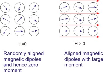
In paramagnetic materials, atoms have a permanent non-zero net magnetic moment due to the sum of orbital and spin magnetic moments. However at room temperature, in paramagnetic materials, thermal energy causes random distribution of magnetic moments and hence net magnetization appears to be zero for the whole material (not just an atom).
Upon application of a field, the moments tend to align up in the direction of the field overcoming the thermal barrier and giving a net positive magnetic moment in the direction of the applied field. The susceptibilities of these materials are usually very small, 10-3 to 10-6.
| Figure 6.7 Schematic representation of spins in a paramagnetic solid |
In most solids, only spin paramagnetism is observed, since the electron orbits are considered as coupled to the lattice (the orbital moments are quenched) and hence do not contribute significantly to the magnetic moment. Qualitatively, it is due to the electric field generated by the surrounding ions in the solid. Because of these electric fields, the orbitals are strongly coupled to the lattice and hence cannot reorient themselves along the field and therefore, do not contribute towards the magnetic moment. On the other hand, electron spins are weakly coupled and hence form a major part of the magnetic moment.
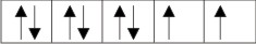
Spin paramagnetism is observed in materials with unfilled d-shells which follow Hund’s rule which says that in the partially filled d-orbitals, the moment is maximized by the first filling all the spin states of one direction followed by filling in other direction.
For example, Ni, with an atomic number of 28 has an electronic configuration of 1s2, 2s2, 2p6, 3s2, 3p6,4s2 and 3d8. The filling in of partially occupied d-orbital is achieved as follows:
As a result, each Ni atom has a net magnetization of 2μB.
Exception to this may be rare-earth elements and their derivatives which have deep-lying 4f- electrons. These are shielded by the outer electrons from the crystal field and as result they show both spin and orbital paramagnetism.
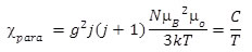
Susceptibility (from orbital moment) in paramagnetic material shows temperature dependence as governed by Curie’s law and is given as
where N is the number of atoms per unit volume, μm is the magnetic moment of an atom and C is Curie constant. Curie’s law states that susceptibility of a paramegntic material is inversely proportional to temperature.
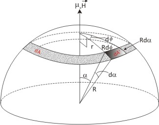
The derivation for Equation (6.22) is quite similar to what we did for dipolar polarization in module 4 .Here we assume that each atom has a magnetic moment μm whose magnitude is the same but the direction can be random. The magnetic energy in a field B would be μm.B = -μmB cosα where α is the angle between the moment and field.
| Figure 6.8 Representation of magnetic moment in a paramagnetic solid with respect to the applied field |
Boltzmann statistics in classical thermodynamics gives the probability of having any angle i.e. of occupying any energy as exp(-μmH.cosα/kT). As a result, as you can also notice that it is more plausible to have moment closer to 0° than 180° with respect to the applied field, simply because that leads to smaller energy than those at 180°.
Consider a smaller number of dipoles dn making an angle a with respect to the applied field and penetrating an area dA as shown in figure 6.8 which is proportional to exp(-μmHcosα/kT)
Considering a unit radius of the sphere (R=1), the area dA can be worked out as
Hence dn can be expressed as
or
dn =  |
|
where C is a constant.
Assuming that γ = μmH/kT, we can integrate equation (6.24) for a between 0 to 180º which will yield the total number of dipoles i.e.
Now, the total magnetic moment along the direction of magnetic field can be expressed multiplication of number dipoles multiplied by the magnetic moment of each dipole along the field direction (μmcosα) and is given as
Dividing equation (6.25) by (6.26) yields the average magnetization, Mavj, as
Now, following a similar procedure as in Module 4 for orientation polarization, we can show that for reasonably small magnetic field, moments are parallel to applied field and magnetization M can be expressed as
where β =(μmB)(kT) and L(β) = cot hβ - 1/β is called Langevin function. For most cases i.e. when μmB << kT, ,we can assume L(β) = β/3. Using this approximation, we can write equation (6.28) as
OR
where Curie constant C = (Nμm2 μ0)/3k .
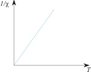
| Figure 6.9 Susceptibility vs temperature plot for a paramagnetic material |
Equations (6.29 and 6.30) show that induced magnetization is proportional to the applied field and is larger at lower temperature. The same result can also be shown using quantum mechanism which is not a part of this course.
Quantum mechanics, for any characteristic number j (could be combined for both orbital and spin moments or only s for spin moments), also gives
which is similar to (6.29) with  . Here, g is Landé-g factor. . Here, g is Landé-g factor.
The theoretically derived and experimentally obtained values of magnetic moment for a few selected magnetic ions are given below and here, you can see while for rare earth ions total magnetic moment value gives a much better estimate, for transition elements, spin only magnetism in a better estimate (Reference: Introduction to Solid State Physics, C. Kittel).
| Ion |
Configuration |
Calculated |
Measured |
| |
|
 |
 |
 |
Rare Earths |
| Ce3+ |
 |
|
- |
2.4 |
| Pr3+ |
 |
|
- |
3.5 |
| Nd3+ |
 |
|
- |
3.5 |
Transition Elements |
| Mn3+ |
 |
0.00 |
4.90 |
4.9 |
| Mn2+, Fe3+ |
 |
5.92 |
5.92 |
5.9 |
| Fe2+ |
 |
6.70 |
4.90 |
5.4 |
| Co2+ |
 |
6.63 |
3.87 |
4.8 |
| Ni2+ |
 |
5.59 |
2.83 |
3.2 |
|