Rayleigh scattering (contd..)
A typical intensity fluctuation recorded in a fluid medium at thermal equilibrium is shown in Figure 7.7. Statistical analysis is possible only for stationary signals for which the time-average is clearly defined (refer module 1 for a longer discussion on signal analysis). Hence, dynamic scattering measurements are to be carried out under constant density (meaning, constant temperature and pressure) conditions, at least for the duration of the experiment. The light intensity signals relate to random density fluctuations. Figure 7.7 also shows the normalized autocorrelation function  of the density fluctuations. In practice, such quantities are obtained by first calculating the Fourier transform of the time series (see module 1). The timescale of the density fluctuations. In practice, such quantities are obtained by first calculating the Fourier transform of the time series (see module 1). The timescale  associated with the fluctuations can be determined as the intercept of the slope of with the time axis. Hence associated with the fluctuations can be determined as the intercept of the slope of with the time axis. Hence
The thermal diffusivity of the liquid medium is then obtained from classical heat conduction (applied to thermal fluctuations) as
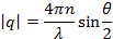
where  is the scattering vector is the scattering vector
Here,  is the wavelength of the incident light, n is the refractive index of the medium, and θ is the angle between the scattering vector and the incident light vector. The refractive index as well as the scattering angle has to be determined as a part of the experiment. is the wavelength of the incident light, n is the refractive index of the medium, and θ is the angle between the scattering vector and the incident light vector. The refractive index as well as the scattering angle has to be determined as a part of the experiment.
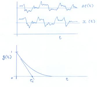
Figure 7.7: Light intensity and density fluctuations recorded during a dynamic light scattering experiment. The graph below is a plot of autocorrelation as a function of time delay, with representing the decay rate of the autocorrelation function.
|